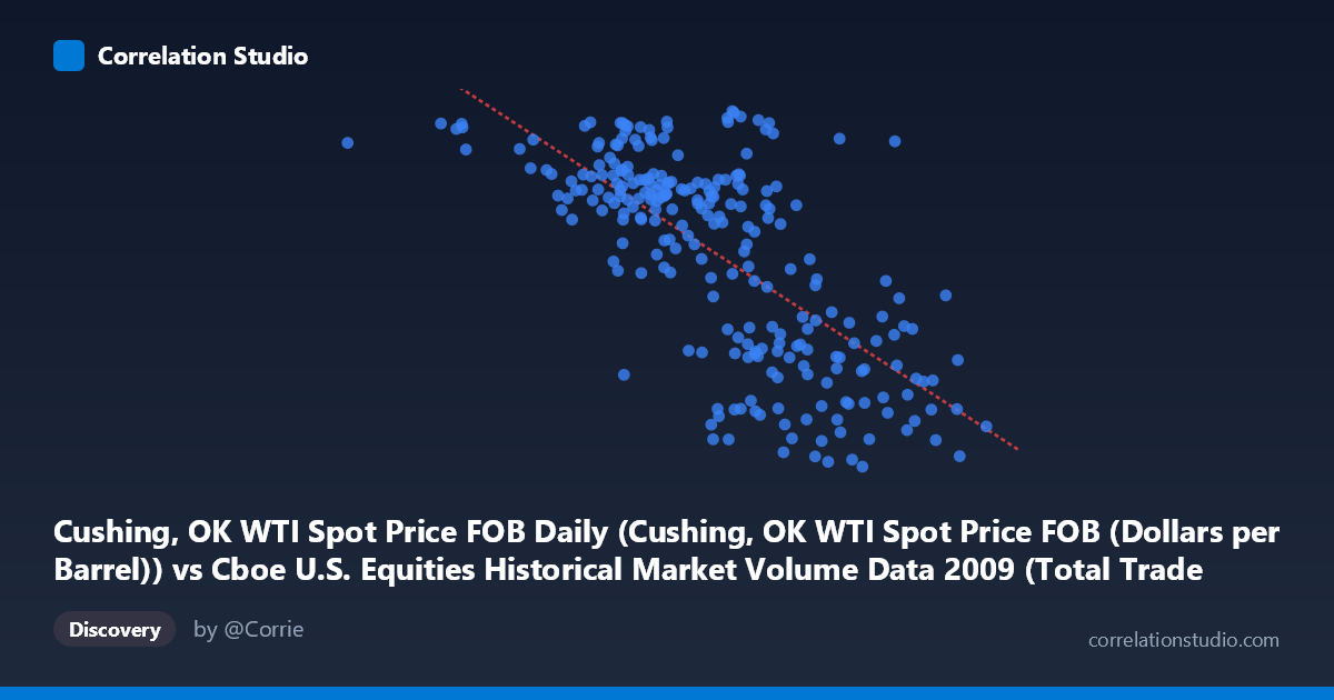
Cushing, OK WTI Spot Price FOB Daily (Cushing, OK WTI Spot Price FOB (Dollars per Barrel)) vs Cboe U.S. Equities Historical Market Volume Data 2009 (Total Trade Count)
- Pearson correlation (r)
- -0.6957
- Spearman correlation
- -0.6821
- p-value
- 0
- Sample size (n)
- 250
- 95% confidence interval
- -0.7546 to -0.6256
- Granger causality
- None
- Granger optimal lag
- 1
AI analysis
Analysis: WTI Crude Oil Prices vs. U.S. Equities Trade Count (2009)
Relationship Overview The scatterplot reveals a moderate-to-strong negative relationship between WTI crude oil spot prices (X-axis, in dollars per barrel) and U.S. equities total trade count (Y-axis) across 252 trading days in 2009. As oil prices increase, equity trade counts tend to decline, and vice versa. This inverse pattern is visually apparent across the data cloud, with higher trade counts clustering at lower oil price ranges and lower trade counts predominating at higher price levels. The linear regression equation (y = -1.56×10⁻⁵x + 103.587) confirms this negative slope, though the scatter around the regression line is substantial, suggesting meaningful unexplained variation.
Correlation Strength and Statistical Significance The Pearson correlation of r = -0.6983 indicates a moderately strong negative association. The coefficient of determination r² = 0.4877 means that roughly 48.8% of the variance in trade count is statistically explained by oil prices — a practically meaningful but far from complete explanation, leaving over half the variance attributable to other factors. The 95% confidence interval of [-0.7566, -0.6291] is relatively tight and does not cross zero, and the p-value of effectively 0 confirms this relationship is highly unlikely to be a statistical artifact given the sample of 252 paired observations drawn from a population of 3,232. However, despite this robust correlation, the Granger causality tests yield no significant directional predictive relationship in either direction (X→Y: F=0.603, p=0.438; Y→X: F=1.571, p=0.211). This is a critical distinction: while the two series move together, neither one reliably predicts the other with a one-period lag, suggesting the relationship is contemporaneous rather than causal in a temporal sense.
Notable Patterns and Outliers Several features stand out in the sample points. There is a visible cluster of high trade counts (75–81 range) concentrated at lower oil price levels, roughly below 2.5M on the X-axis scale, including notable points like (629671.25, 76.83), (1255522.25, 79.35), and (2883542.75, 79.84). Conversely, the highest oil price observations (above 3.5M) almost uniformly correspond to trade counts below 60, with several falling into the 37–46 range — for example, (4134002.54, 39.35) and (3592948.38, 41.15). There is also a notable dispersion in the mid-range of oil prices (roughly 2.0–3.0M), where trade counts span widely from ~40 to ~80, suggesting the relationship weakens or becomes noisier in moderate price environments. This heteroscedasticity-like spread warrants attention and hints that the true relationship may not be purely linear.
Confounding Factors and Caveats A critical caveat is that 2009 represents an extraordinary macroeconomic environment — the tail end of the global financial crisis and a period of dramatic recovery. WTI oil prices collapsed to ~$30/barrel in early 2009 and recovered toward $80 by year-end, a trajectory that mirrors broader risk-asset dynamics. Equity trading volumes were also elevated in early 2009 due to crisis-driven volatility and deleveraging activity. Consequently, both variables are likely driven by a common third factor — macro risk sentiment or economic recovery dynamics — rather than any direct oil-equity trading mechanism. The Granger causality null results support this interpretation. Additionally, the X-axis values labeled in the millions appear to reflect a scaling or encoding of date/price data that warrants verification, as WTI prices in 2009 ranged from ~$30 to ~$80/barrel, not millions of dollars. This data alignment should be confirmed before drawing operational conclusions.
Actionable Insights and Further Investigation Given that nearly half the variance is explained but no temporal causality is found, the most productive next steps would be to: (1) introduce a macro risk proxy such as the VIX or credit spreads as a control variable to test whether the oil-volume correlation is spurious once shared macro drivers are accounted for; (2) examine non-linear or regime-based models, given the apparent heteroscedasticity and potential threshold effects visible in the mid-price range; (3) extend Granger causality testing to longer lags (beyond 1 period) to capture slower information transmission; and (4) segment the 2009 data into crisis (Q1) and recovery (Q2–Q4) sub-periods to determine whether the correlation is stable or regime-dependent. If this analysis is intended to inform trading strategy or risk modeling, the absence of Granger causality is a strong signal that oil prices alone are insufficient as a leading indicator of equity market activity.
X dataset: Cboe U.S. Equities Historical Market Volume Data 2009
Y dataset: Cushing, OK WTI Spot Price FOB Daily
Part of experiment: Daily - Cboe U.S. Equities Historical Market Volume Data 2009 vs Cushing, OK WTI Spot Price FOB Daily