Personal Consumption Expenditures: Chain-type Price Index Less Food and Energy (JCXFE) | FRED | St. Louis Fed (JCXFE) vs FRED – Copper Price (Global) (PCOPPUSDM)
- Pearson correlation (r)
- 0.8527
- Spearman correlation
- 0.7979
- p-value
- 0
- Sample size (n)
- 139
- 95% confidence interval
- 0.7998 to 0.8925
- Granger causality
- None
- Granger optimal lag
- 1
- Time coverage
- 1992-01-01 to 2026-07-01
- Recomputed on refreshed data
- 2026-10-31 (r was 0.8462)
AI analysis
Analysis: Copper Prices vs. Core PCE Price Index
1. Relationship Overview
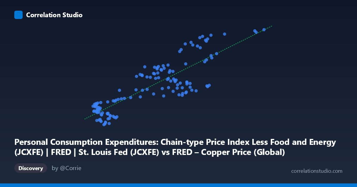
The scatterplot reveals a strong positive, largely linear relationship between global copper prices (X) and the core PCE price index (Y, ex-food and energy). As copper prices rise from roughly $1,400 to $13,000/metric ton, the core PCE index climbs steadily from around 64 to 129. The regression line (y = 0.00489x + 63.99) fits the data reasonably well across most of the range, though the relationship shows some heteroskedasticity — scatter around the trend line widens somewhat in the mid-range (X ≈ 6,000–9,000), suggesting other factors modulate the relationship at certain price levels.
2. Strength, Direction, and Statistical Confidence
The correlation coefficient (r = 0.84) indicates a strong positive association, with r² = 0.705 meaning roughly 70% of the variance in core PCE can be statistically explained by copper price movements alone — a substantial share for a two-variable macroeconomic relationship. The 95% confidence interval [0.782, 0.883] is tight and entirely excludes weak or negative correlations, and the p-value of ~0 confirms this relationship is highly unlikely to be due to chance. However, the Granger causality tests are important context: neither variable significantly predicts the other at a 1-period lag (X→Y: p=0.87; Y→X: p=0.75). This means that despite the strong contemporaneous correlation, there's no evidence that copper price changes temporally precede and forecast core inflation changes (or vice versa) in this dataset — the relationship appears to be coincident rather than predictive, likely both responding to a common underlying driver (e.g., broad macroeconomic expansion, monetary policy, or global demand cycles).
3. Notable Patterns and Outliers
The data shows a fairly consistent upward trend, but a few features stand out: at the low end (X < 2,500), Y values cluster tightly between 63–80, showing low scatter and a clean relationship. In the mid-range (X ≈ 6,000–8,500), there is more dispersion — points like (7,726.74, 84.43) and (7,980.93, 86.15) sit notably below the trend line, while (7,941.36, 120.40) and (8,976.68, 125.00) sit well above it, indicating episodes where copper prices moved without proportional inflation response (or with a lag). The highest copper price point (12,986.61, 128.92) extrapolates well with the trend, suggesting the relationship may hold at the extremes, though this is a single point with no neighboring data to confirm curvature.
4. Confounding Factors and Caveats
Both series are likely non-stationary trending time series (inflation indices and commodity prices both generally rise over multi-decade periods), which is a classic setup for spurious correlation — two unrelated trending variables can show high r² simply because both increase over time. The Granger causality results reinforce this concern: the lack of predictive power in either direction is consistent with two variables driven by a shared macro trend (e.g., global growth, USD strength, or general price-level inflation) rather than a direct causal link between copper specifically and core consumer prices. Additionally, "core" PCE deliberately excludes energy, so any copper-inflation transmission would run through indirect channels (industrial/construction costs, capital goods pricing) rather than direct commodity pass-through.
5. Suggestions for Further Investigation
To move beyond the correlation/causation ambiguity, analysts should: (1) test both series for unit roots (e.g., ADF test) and, if non-stationary, examine cointegration or use differenced/detrended series to rule out spurious trend correlation; (2) extend the Granger test to multiple lag lengths (quarters/years) since monetary and industrial pass-through effects may take longer than one period; (3) control for a shared common driver — such as global industrial production, GDP growth, or a broad commodity index — to see if copper's explanatory power holds up in a multivariate regression; and (4) consider copper as a leading indicator candidate only if longer-lag Granger tests or cross-correlation analysis show stronger directional signal, since the current single-lag test does not support using copper prices as a standalone inflation forecasting tool.
X dataset: FRED – Copper Price (Global)
Y dataset: Personal Consumption Expenditures: Chain-type Price Index Less Food and Energy (JCXFE) | FRED | St. Louis Fed
Part of experiment: Copper - FRED – Copper Price (Global) vs Personal Consumption Expenditures: Chain-type Price Index Less Food and Energy (JCXFE) | FRED | St. Louis Fed