Bitcoin Historical Data (2010-2024) (HashRate) vs CryptoDataDownload – Binance BTC/USDT Daily OHLCV (High)
- Pearson correlation (r)
- 0.8894
- Spearman correlation
- 0.88
- p-value
- 0
- Sample size (n)
- 3191
- 95% confidence interval
- 0.8819 to 0.8964
- Granger causality
- None
- Granger optimal lag
- 10
AI analysis
Analysis: Bitcoin Hash Rate vs. Price (High)
1. Overview of the Relationship
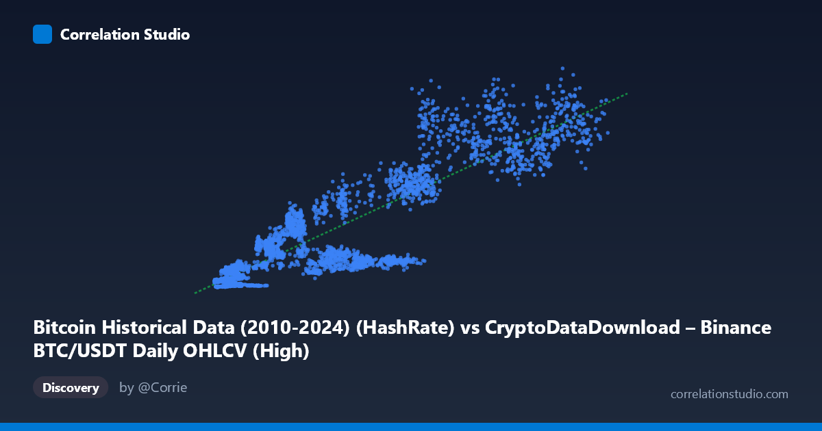
The scatterplot shows a strong positive association between Bitcoin's network hash rate (X) and its daily high price (Y). As hash rate increases across its range (~3,277 to ~126,200 units), price highs climb from single-digit millions to over $1.3 billion in this scaled representation. The relationship is not perfectly linear—it appears to follow a pattern with increasing variance (heteroscedasticity) at higher hash rate values, where price outcomes become more dispersed for similar hash rate levels.
2. Strength, Direction, and Statistical Confidence
The correlation coefficient (r = 0.8894) indicates a strong positive linear relationship, with r² = 0.7909 meaning approximately 79% of the variance in price highs is statistically explained by hash rate alone. The tight 95% confidence interval [0.8819, 0.8964] combined with a p-value of 0 (effectively p < 0.001) confirms this correlation is highly reliable and not a product of chance, given the large sample size (n = 3,191).
However, the Granger causality results substantially temper any causal interpretation: neither variable significantly predicts the other in a temporal/leading sense (X→Y: p = 0.469; Y→X: p = 0.121). This suggests the strong contemporaneous correlation likely reflects a shared underlying driver (e.g., overall market cycle, mining profitability incentives, adoption trends) rather than hash rate directly causing price movements or vice versa in a lagged, predictive sense.
3. Notable Patterns and Outliers
Several features stand out: - Fan-shaped dispersion: At low hash rates (<20,000), price highs are tightly clustered near the lower end (under $250M scaled), but as hash rate rises above 60,000–90,000, price highs vary widely (from ~$150M to over $1.1B), suggesting other factors increasingly influence price at higher network maturity. - Possible plateau/saturation: Some high-hash-rate points (e.g., ~84,000–90,000) show similar price levels, hinting at diminishing marginal price response to hash rate increases—consistent with a logarithmic or S-curve relationship rather than pure linearity. - Low outliers: A few points with moderate hash rate (~55,000–60,000) show comparatively low prices (~$118M–$159M), diverging from the general trend—these may correspond to specific market corrections or bear-market periods where hash rate lagged price crashes.
4. Confounding Factors and Caveats
This relationship is likely confounded by time itself: both hash rate and price have historically trended upward over Bitcoin's lifecycle (2017–2026 coverage), so the correlation may partly reflect a shared secular growth trend rather than a direct mechanical link. Key confounders include: - Market cycles: Bull/bear regimes affect price independently of mining activity. - Mining economics: Hash rate is influenced by electricity costs, ASIC efficiency, and regulatory shifts (e.g., China's 2021 mining ban), which are unrelated to price demand. - Lag effects: Miners often adjust hash rate in response to past price changes (profitability-driven), while price also responds to speculative/macro factors independent of hash rate—the lack of Granger causality is consistent with this bidirectional, non-simple lag structure.
5. Actionable Insights and Further Investigation
Given r² of 79%, hash rate is a useful but incomplete linear predictor of price—supplementing models with macro variables (interest rates, exchange volume, on-chain metrics like active addresses) would likely improve explanatory power. Since Granger tests show no clear predictive direction, avoid using hash rate as a leading indicator for price trading strategies; instead, treat both as co-evolving with the market cycle. Further work should: - Test log-transformed variables to check if the relationship is better modeled as exponential/power-law (common in Bitcoin network metrics). - Segment the analysis by market regime (bull/bear/sideways) to see if correlation strength or slope differs. - Explore lagged cross-correlation at finer granularity (daily/weekly) beyond the 10-period Granger lag to detect any short-term lead-lag dynamics obscured by data aggregation.
X dataset: CryptoDataDownload – Binance BTC/USDT Daily OHLCV
Y dataset: Bitcoin Historical Data (2010-2024)
Part of experiment: Bitcoin - CryptoDataDownload – Binance BTC/USDT Daily OHLCV vs Bitcoin Historical Data (2010-2024)