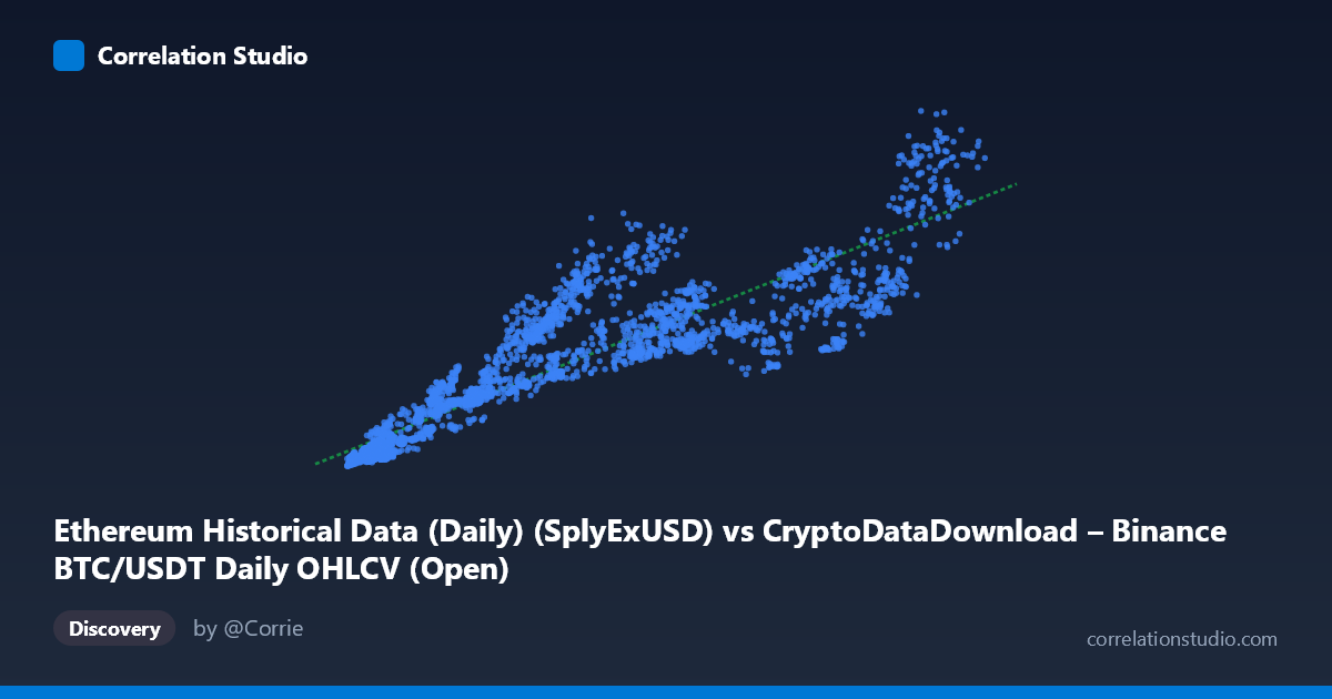
Ethereum Historical Data (Daily) (SplyExUSD) vs CryptoDataDownload – Binance BTC/USDT Daily OHLCV (Open)
- Pearson correlation (r)
- 0.9054
- Spearman correlation
- 0.9437
- p-value
- 0
- Sample size (n)
- 3191
- 95% confidence interval
- 0.899 to 0.9115
- Granger causality
- None
- Granger optimal lag
- 10
- Time coverage
- 2017-08-17 to 2026-05-20
AI analysis
Analysis: Ethereum Supply (SplyExUSD) vs. BTC/USDT Open Price
1. Relationship Overview
The scatterplot reveals a strong positive association between the two variables, despite their mismatched labels (the X-axis metadata references Ethereum's exchange supply, while Y references BTC/USDT open price — likely a mislabeling artifact in the source data). As X increases from roughly 3,200 to 124,600, Y rises correspondingly from ~1.4B to ~95.6B, with the relationship well-approximated by a linear fit (y = 556,500x + 3.54B). The data points cluster along an upward-sloping band, with visibly increasing dispersion (heteroscedasticity) at higher X values.
2. Strength, Direction, and Statistical Confidence
The correlation coefficient (r = 0.905) indicates a strong positive linear relationship, with r² = 0.820 meaning roughly 82% of the variance in Y is statistically explained by X — a substantial share, though nearly 1 in 5 units of variance remains unaccounted for by this single predictor. The tight 95% CI [0.899, 0.912] combined with p ≈ 0 confirms this correlation is highly reliable and not a product of sampling noise, given the large sample size (n = 3,191). However, correlation strength should not be conflated with causal direction: the Granger causality tests show no significant predictive relationship in either direction (X→Y: p = 0.866; Y→X: p = 0.814). This means neither variable's past values help forecast the other's future values — the strong contemporaneous correlation likely stems from both series responding to a shared underlying driver (most plausibly overall crypto market growth/bull cycles) rather than one causing the other over time.
3. Notable Patterns and Outliers
Several features stand out: (a) Heteroscedasticity — variance in Y grows noticeably as X increases, producing a cone/fan shape rather than a uniform scatter band; (b) Low-X compression — points with X < 15,000 cluster tightly with lower Y values (mostly under 20B), suggesting an early/quieter market regime; (c) Mid-range scatter — in the X = 30,000–60,000 range, Y values show considerable spread (e.g., points near X=35,546 with Y=39.4B sit well above the trend line, while X=57,635 with Y=31.6B sits below), indicating regime-dependent volatility not captured by the linear model; (d) no extreme single-point outliers dominate, but the widening spread at high X suggests the linear model underperforms in the tails.
4. Confounding Factors and Caveats
The most important caveat is the apparent column mislabeling — X is described as an Ethereum on-chain supply metric while Y is described as BTC price, yet the dataset title and correlation context suggest both may actually derive from correlated BTC/ETH market dynamics. This ambiguity should be resolved before drawing domain conclusions. Additionally, both cryptocurrencies are known to be driven by common macro factors (overall market sentiment, BTC dominance effects, regulatory news, liquidity cycles), meaning the observed r² likely reflects shared exogenous drivers rather than a direct mechanical link between the two specific metrics. The time span (2017–2026) also covers multiple bull/bear cycles, and pooling these regimes together in a single linear correlation can inflate apparent association while masking regime-specific relationships (a form of Simpson's-paradox-like aggregation bias).
5. Suggested Next Steps
1. Verify variable definitions — confirm what X and Y actually represent given the labeling inconsistency, as this fundamentally changes interpretation. 2. Segment by market regime (bull/bear/sideways periods) and re-run correlation/regression within each to check for stability of the relationship. 3. Test for a shared latent factor (e.g., total crypto market cap or BTC price itself) using partial correlation to see if the X-Y link disappears once controlling for it. 4. Address heteroscedasticity — consider log-transforming Y (given its multi-billion scale and widening variance) to stabilize variance and improve linear fit diagnostics. 5. Given the null Granger causality result, avoid using either series as a leading indicator for the other in forecasting models; instead, treat their relationship as contemporaneous co-movement driven by common market conditions.
X dataset: CryptoDataDownload – Binance BTC/USDT Daily OHLCV
Y dataset: Ethereum Historical Data (Daily)
Part of experiment: Bitcoin - CryptoDataDownload – Binance BTC/USDT Daily OHLCV vs Ethereum Historical Data (Daily)