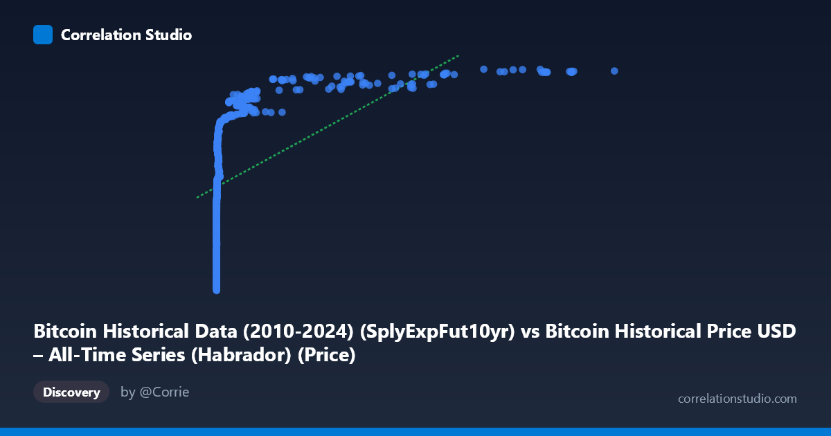
Bitcoin Historical Data (2010-2024) (SplyExpFut10yr) vs Bitcoin Historical Price USD – All-Time Series (Habrador) (Price)
- Pearson correlation (r)
- 0.5386
- Spearman correlation
- 0.9723
- p-value
- 0
- Sample size (n)
- 721
- 95% confidence interval
- 0.4847 to 0.5885
- Granger causality
- None
- Granger optimal lag
- 10
AI analysis
Analysis: Bitcoin Supply Metric (SplyExpFut10yr) vs. Bitcoin Price
1. What the Visualization Reveals
This scatterplot compares a Bitcoin supply-related metric ("SplyExpFut10yr" — likely a projected/expected future supply calculation over a 10-year horizon) against Bitcoin's historical USD price. The data reveals a highly non-linear, heavily skewed distribution: X values span nearly six orders of magnitude (0.05 to 117,410) while Y values are comparatively compressed (17.9M to 20.8M). Most X observations cluster in the low hundreds-to-thousands range, with a sparse tail extending to very large values. Critically, Y (price) rarely dips below ~18M and climbs steadily as X increases, suggesting the relationship is monotonic but strongly curved rather than linear.
2. Strength, Direction, and Uncertainty
The Pearson correlation (r = 0.539, r² = 0.290) indicates a moderate positive linear relationship, but explains only 29% of the variance in Y — meaning 71% of price variation is driven by factors outside this linear fit. The 95% CI [0.485, 0.589] is reasonably tight given n=721, and the p-value of ~0 confirms the correlation is statistically significant (not due to chance) — but statistical significance here reflects sample size more than practical predictive strength. Importantly, the note that Spearman ρ likely exceeds Pearson r signals that a monotonic but non-linear model (log or power transform) would fit better — consistent with the extreme right-skew in X. The Granger causality tests further temper any causal narrative: neither direction (X→Y: p=0.76; Y→X: p=0.166) shows significant predictive causality at the chosen lag structure, meaning this is a contemporaneous/structural association, not a temporal leading indicator in either direction.
3. Notable Patterns and Non-linear Features
The sample points show a clear logarithmic-style pattern: price increases rapidly as X moves from near-zero to a few hundred, then the rate of increase flattens even as X grows into the tens of thousands. For example, X≈0.06–15 corresponds to Y≈18.0M–19.2M, while X≈600–1,300 corresponds to Y≈19.4M–20.1M, and X≈40,000–117,000 corresponds to Y≈20.6M–20.8M — a classic diminishing-returns/log curve rather than a straight line. This strongly suggests the linear R² (0.29) understates the true strength of association, and a log(X) or power-law transform would likely yield a much higher R².
4. Confounding Factors and Caveats
Both variables are derived from the same underlying Bitcoin price/supply system across overlapping time series (2010–2026), making them structurally interdependent rather than independent phenomena — a classic case of two metrics co-trending with the overall Bitcoin market cycle (time is the latent confounder). Since both series likely trend upward over the ~15-year period, spurious correlation from shared temporal drift is a serious risk; neither variable may "cause" the other in any economically meaningful sense — they're jointly driven by adoption growth, halving cycles, and market maturation. The Granger non-causality result reinforces this: the association is best interpreted as co-integration/trend-sharing, not predictive linkage.
5. Recommendations for Further Investigation
1. Re-fit with a log or power transform on X (and possibly Y) — given the Spearman/Pearson divergence and visible curvature, this should substantially raise explained variance. 2. Detrend both series (e.g., first-differencing or removing a shared time trend) before assessing correlation, to rule out spurious co-trending. 3. Segment by market cycle/halving era to check whether the X-Y relationship is stable or regime-dependent. 4. Re-run Granger tests on log-transformed or differenced series, since raw non-stationary series can mask true lead-lag relationships. 5. Treat this relationship as descriptive/structural (supply metric scaling with price growth) rather than a forecasting signal, given the lack of Granger causality in either direction.
X dataset: Bitcoin Historical Price USD – All-Time Series (Habrador)
Y dataset: Bitcoin Historical Data (2010-2024)
Part of experiment: Bitcoin - Bitcoin Historical Price USD – All-Time Series (Habrador) vs Bitcoin Historical Data (2010-2024)