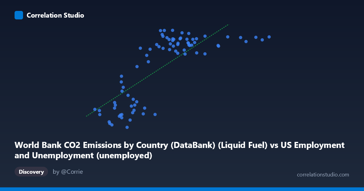
World Bank CO2 Emissions by Country (DataBank) (Liquid Fuel) vs US Employment and Unemployment (unemployed)
- Pearson correlation (r)
- 0.7729
- Spearman correlation
- 0.754
- p-value
- 0
- Sample size (n)
- 80
- 95% confidence interval
- 0.6664 to 0.8486
- Granger causality
- None
- Granger optimal lag
- 10
AI analysis
Scatterplot Analysis: Liquid Fuel CO2 Emissions vs. US Unemployment
1. Overall Relationship Pattern
The scatterplot reveals a moderately strong positive relationship between World Bank liquid fuel CO2 emissions and US unemployment figures across the 1941–2020 time period. However, the relationship is notably non-linear: the data exhibits a pronounced sigmoid or plateau curve, where unemployment rises steeply as emissions increase from low values (roughly 670–6,000 units), then flattens and saturates at higher emission levels (above ~7,000 units), where unemployment clusters tightly around 11,000–13,600 regardless of further emission increases. A simple linear regression (y = 0.910x + 3,788) thus captures the broad trend but misrepresents the true functional form.
2. Correlation Strength, Direction, and Causal Framing
The Pearson correlation of r = 0.773 indicates a moderately strong positive association, and the R² = 0.597 tells us that approximately 59.7% of the variance in US unemployment is statistically explained by liquid fuel CO2 emissions — a meaningful but far from complete accounting, leaving roughly 40% of variation unexplained by this single predictor. The 95% confidence interval for r of [0.666, 0.849] is reasonably tight and excludes zero, and the p-value of effectively 0 confirms this correlation is highly statistically significant at any conventional threshold (N = 86, n = 80 paired observations). Despite this statistical significance, the Granger causality analysis delivers a critical tempering result: neither direction shows significant temporal predictive power (X→Y: F = 0.41, p = 0.94; Y→X: F = 1.71, p = 0.11, both non-significant at the optimal 10-period lag). This means that knowing past values of CO2 emissions does not help predict future unemployment beyond its own history, and vice versa — the correlation is real but lacks temporal predictive directionality, strongly suggesting a shared common driver rather than any direct causal link.
3. Notable Patterns, Clusters, and Outliers
Several structural features stand out upon close inspection:
- Lower-left cluster (emissions < ~4,000; unemployment < ~6,000): These likely represent early decades (1940s–1960s) when both industrial activity and unemployment were at lower absolute scales. A few points here appear to deviate notably — for instance, (3288, 2497) and (5560, 3972) sit unusually low in unemployment relative to their emission levels, potentially representing recession or wartime anomalies. - Upper saturation plateau (emissions ~6,000; unemployment ~11,000–13,600): A dense cluster where unemployment appears largely decoupled from further emission increases, suggesting a ceiling effect or structural change in labor markets. - Transitional zone (~4,000–6,500 emissions): The steepest part of the curve, where unemployment increases most rapidly — this is where the linear model's approximation is most reasonable. - High-emission outliers — points at (14,825; 12,848) and (13,747; 12,804) represent the far right tail, likely recent decades with high fossil fuel use, yet unemployment is not commensurately extreme. - Point (3288, 2497) is the minimum Y value and is a notable outlier below the general trend, possibly corresponding to a specific low-unemployment year in an early period.
4. Confounding Factors and Interpretive Caveats
The correlation almost certainly reflects shared temporal trends rather than any meaningful mechanistic link between liquid fuel CO2 emissions and unemployment. Both variables are strongly driven by macroeconomic growth cycles and population expansion over the 80-year span: as the US economy and population grew, both total employment (and thus the absolute number of unemployed workers) and energy consumption increased together. Key confounders include:
- Population growth: More people means both more workers (raising the unemployment count even at stable rates) and more fuel consumption. - Economic expansion: GDP growth drives both industrial fuel use and labor market scale simultaneously. - Structural labor market changes: The nature of unemployment (cyclical vs. structural vs. frictional) shifted dramatically across 1941–2020, including wartime mobilization, deindustrialization, and the 2008 and 2020 crises. - Measurement mismatch: The dataset labels suggest a potential column-dataset mismatch (X is labeled as coming from US Employment data but measures CO2; Y from World Bank CO2 data but measures unemployment), which warrants careful verification of data provenance before drawing any conclusions. - The non-linearity means the reported linear R² of 0.597 overstates predictive fit in the extremes while understating it in the transition zone.
5. Actionable Insights and Further Investigation
Given the non-causal, trend-driven nature of this correlation, the most productive next steps would be:
- Detrend both series (e.g., first-differencing or per-capita normalization) to remove shared population/GDP growth and test whether any residual correlation persists — this would reveal whether the relationship holds beyond common temporal drift. - Use unemployment rate (%) rather than absolute unemployed count to control for labor force size, which would likely substantially weaken or eliminate the correlation. - Segment the analysis by decade to test whether the relationship is stable across time or is entirely an artifact of the post-WWII growth era. - Fit a non-linear model (logistic or piecewise regression) to better capture the evident saturation curve and obtain more honest goodness-of-fit estimates. - Introduce mediating variables such as GDP, population, or energy intensity to formally test whether the apparent relationship is entirely explained by shared confounders through a multivariate or path analysis framework.
In summary, while the r = 0.773 correlation is statistically robust, the absence of Granger causality in either direction, the evident non-linearity, and the strong likelihood of shared temporal confounders collectively indicate that this relationship should not be interpreted causally — it is a spurious correlation of two quantities that both grew with the modern US economy over eight decades.
X dataset: US Employment and Unemployment
Y dataset: World Bank CO2 Emissions by Country (DataBank)
Part of experiment: Yearly - US Employment and Unemployment vs World Bank CO2 Emissions by Country (DataBank)