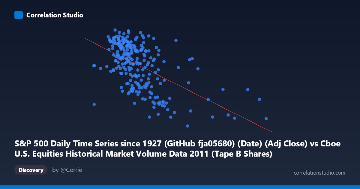
S&P 500 Daily Time Series since 1927 (GitHub fja05680) (Date) (Adj Close) vs Cboe U.S. Equities Historical Market Volume Data 2011 (Tape B Shares)

Pearson correlation (r): -0.5574
Spearman correlation: -0.5372
p-value: 0
Sample size (n): 252
95% confidence interval: -0.6371 to -0.466
Granger causality: None
Granger optimal lag: 1

AI analysis

Analysis: S&P 500 Adjusted Close vs. Cboe Tape B Shares (2011)

Relationship Overview The scatterplot reveals a moderate negative relationship between the S&P 500 adjusted closing price (X-axis) and Cboe Tape B share volume (Y-axis) across 252 trading days in 2011. As the S&P 500 price level rises, Tape B share volume tends to decline, and conversely, volume spikes tend to coincide with lower index levels. This inverse pattern is consistent with a well-documented market phenomenon: retail and institutional traders often increase trading activity during periods of market stress, volatility, or decline, while calmer, higher-price environments tend to see relatively subdued volume. The linear regression equation (y = −1.059×10⁻⁶x + 1371.6) confirms this negative slope, with the intercept anchoring volume estimates at elevated index levels.

Correlation Strength and Statistical Significance The Pearson correlation of r = −0.5574 indicates a moderate negative association, and the R² of 0.3107 means that roughly 31% of the variance in Tape B share volume is explained by the S&P 500 price level — meaningful, but leaving nearly 70% of variation attributable to other factors. The 95% confidence interval of [−0.6371, −0.4660] is relatively tight and entirely negative, confirming the direction of the relationship with reasonable precision. The p-value of essentially zero (given N = 3,780) provides strong evidence against the null hypothesis of no correlation, though the large population size means even modest effects achieve statistical significance easily. Critically, the Granger causality tests show no significant temporal predictive relationship in either direction (X→Y: F = 0.133, p = 0.716; Y→X: F = 0.015, p = 0.901), meaning that knowing yesterday's S&P 500 price does not meaningfully help predict today's Tape B volume, and vice versa. The correlation is therefore contemporaneous rather than predictive, limiting its actionable forecasting utility.

Notable Patterns, Clusters, and Outliers The data cloud shows notable heteroscedasticity: volume variance is considerably wider at lower S&P 500 price levels (roughly 60–90M range on the X-axis) and compresses somewhat at higher price levels. Several outliers warrant attention — points in the upper-right quadrant (e.g., ~169M shares at ~1,285; ~176M shares at ~1,257) show unexpectedly high volume despite elevated index levels, possibly reflecting specific event-driven trading days. Conversely, a cluster of low-volume observations appears around the 120–190M index price range (e.g., ~1,131 and ~1,161 share counts at prices around 124M–127M), which may correspond to the sharp August 2011 market selloff. The bulk of observations cluster between X = 60M–130M and Y = 1,240–1,350, suggesting the relationship is most consistent in this central range, with the tails showing more dispersion and potential non-linearity.

Confounding Factors and Caveats Several important caveats complicate interpretation. 2011 was an atypical year marked by the U.S. debt ceiling crisis, the S&P sovereign credit downgrade in August, and European debt contagion fears — all of which generated episodic volume spikes that may inflate the apparent inverse relationship. Tape B specifically covers NYSE Arca-listed securities (primarily ETFs and regional exchange stocks), meaning volume dynamics may differ substantially from broader market behavior; ETF volume in particular surges during volatility events, potentially driving much of this correlation. Furthermore, price level alone is an imperfect market state variable — volatility (VIX), bid-ask spreads, and institutional rebalancing cycles likely explain significant portions of the remaining 69% variance. The axes in the sample data also appear transposed in the dataset descriptions (X labeled as Date/Adj Close but containing large integers resembling volume figures), which warrants verification of variable assignment before drawing firm conclusions.

Actionable Insights and Further Investigation Despite the lack of Granger causality, the moderate contemporaneous correlation suggests that volume regime analysis conditioned on market level could be useful for market microstructure research or liquidity modeling. Practitioners should consider adding the VIX or realized volatility as a covariate to determine whether price level retains explanatory power after controlling for volatility — the negative relationship may be largely mediated by volatility rather than price per se. A rolling correlation analysis across different market regimes (pre- and post-August 2011 crisis) would clarify whether this relationship is stable or regime-dependent. Finally, non-linear models (e.g., piecewise regression or GAMs) may better capture the apparent heteroscedasticity and threshold effects visible in the scatterplot, potentially improving the explained variance well beyond the current 31%.

X dataset: Cboe U.S. Equities Historical Market Volume Data 2011

Y dataset: S&P 500 Daily Time Series since 1927 (GitHub fja05680) (Date)

Part of experiment: Daily - Cboe U.S. Equities Historical Market Volume Data 2011 vs S&P 500 Daily Time Series since 1927 (GitHub fja05680) (Date)