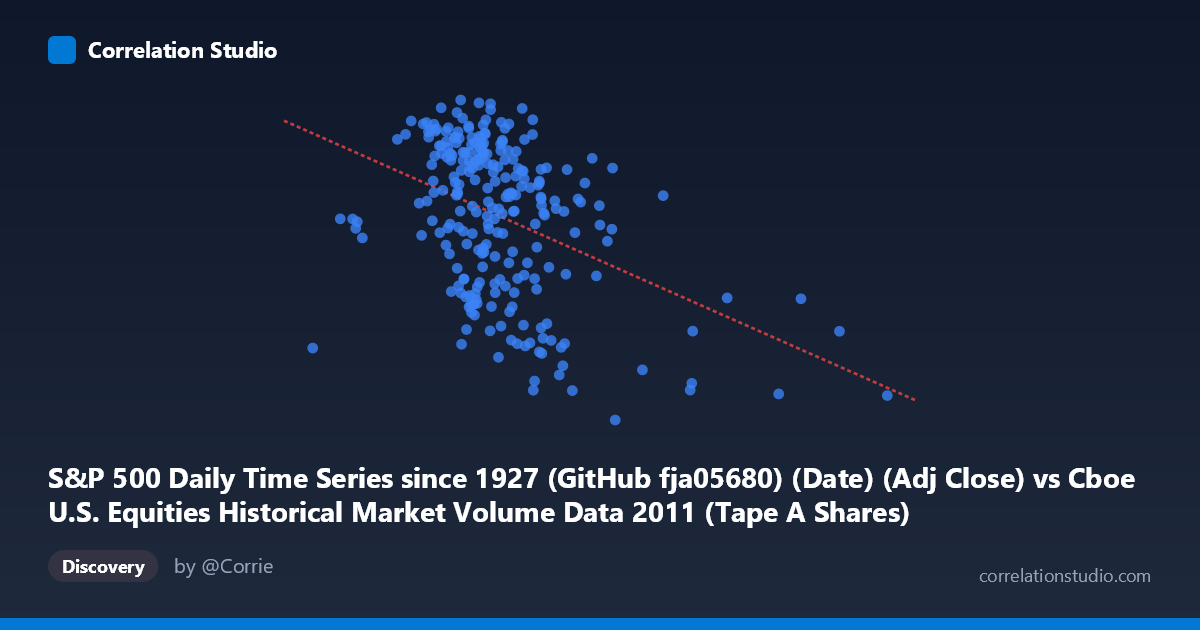
S&P 500 Daily Time Series since 1927 (GitHub fja05680) (Date) (Adj Close) vs Cboe U.S. Equities Historical Market Volume Data 2011 (Tape A Shares)

Pearson correlation (r): -0.4092
Spearman correlation: -0.3745
p-value: 0
Sample size (n): 252
95% confidence interval: -0.5072 to -0.3009
Granger causality: None
Granger optimal lag: 1

AI analysis

Analysis: S&P 500 Adjusted Close vs. Cboe Tape A Share Volume (2011)

Relationship Overview The scatterplot reveals a moderate negative relationship between S&P 500 adjusted closing prices and Cboe Tape A share volume during 2011. As the S&P 500 price level increases, trading volume on Tape A tends to decrease, and conversely, periods of lower index prices correspond with elevated share volume. This inverse pattern is broadly consistent with well-documented market microstructure behavior: heightened volatility and fear-driven selling during market downturns (particularly the mid-2011 correction and debt-ceiling crisis) tend to generate elevated trading activity, while calmer, upward-trending markets often see reduced volume participation.

Correlation Strength and Statistical Significance The Pearson correlation of r = -0.409 indicates a moderate negative association, but the coefficient of determination (r² = 0.1675) tells a more sobering story — only 16.7% of the variance in Tape A share volume is explained by the S&P 500 price level. The remaining ~83% is attributable to other forces entirely. The 95% confidence interval of [-0.507, -0.301] is meaningfully negative throughout, and the p-value of 1.36×10⁻¹¹ confirms this relationship is highly unlikely to be a statistical artifact given n = 252. However, statistical significance here is partly a function of sample size; the effect size itself is modest. Critically, the Granger causality tests show no significant predictive directionality in either direction (X→Y: p = 0.999; Y→X: p = 0.927), meaning that knowing yesterday's S&P 500 price does not help predict today's volume, and vice versa. This absence of temporal precedence rules out a simple lead-lag causal mechanism and suggests the correlation reflects concurrent structural conditions rather than a predictive relationship.

Notable Patterns and Outliers Several features stand out visually. There is a distinct cluster of high-volume observations (X values in the 110M–200M range) concentrated in the lower price range (~1,100–1,200), consistent with the August–October 2011 market selloff triggered by the U.S. credit downgrade. Conversely, observations at higher price levels (300M–450M+) show considerably compressed volume. A handful of outliers appear in the upper-right quadrant — relatively high prices coinciding with unexpectedly elevated volume — which may correspond to specific event-driven days (e.g., options expiration, index rebalancing). The linear regression line (y = -3.81×10⁻⁷x + 1378) captures the central tendency but leaves substantial vertical scatter, suggesting the relationship is heteroscedastic and non-linear components may be present.

Confounding Factors and Caveats Several confounds complicate interpretation. Market regime shifts during 2011 (the European sovereign debt crisis, U.S. debt ceiling standoff, and Fed policy signals) simultaneously suppressed prices and amplified volume, creating a spurious-looking negative correlation that is really a joint response to macro stress events. Seasonality in equity trading (lower summer and holiday volumes) may also independently influence both series. Furthermore, Tape A specifically captures NYSE-listed securities, so compositional changes or exchange competition dynamics (fragmentation to dark pools, alternative venues) could distort volume readings independent of price. The dataset covers only a single calendar year, limiting generalizability.

Actionable Insights and Further Investigation Given the lack of Granger causality, volume should not be used as a predictive signal for price direction in this dataset without additional conditioning variables. Suggested next steps include: (1) segmenting the data by volatility regime (e.g., using VIX thresholds) to test whether the correlation strengthens during stress periods; (2) extending the time horizon beyond 2011 to assess whether the inverse relationship persists across bull and bear cycles; (3) incorporating intraday data or alternative volume metrics (notional value, trade counts) from the same Cboe dataset to triangulate whether the pattern is specific to share count volume; and (4) applying non-linear modeling or regime-switching approaches to better capture the structural breaks visible in the data.

X dataset: Cboe U.S. Equities Historical Market Volume Data 2011

Y dataset: S&P 500 Daily Time Series since 1927 (GitHub fja05680) (Date)

Part of experiment: Daily - Cboe U.S. Equities Historical Market Volume Data 2011 vs S&P 500 Daily Time Series since 1927 (GitHub fja05680) (Date)