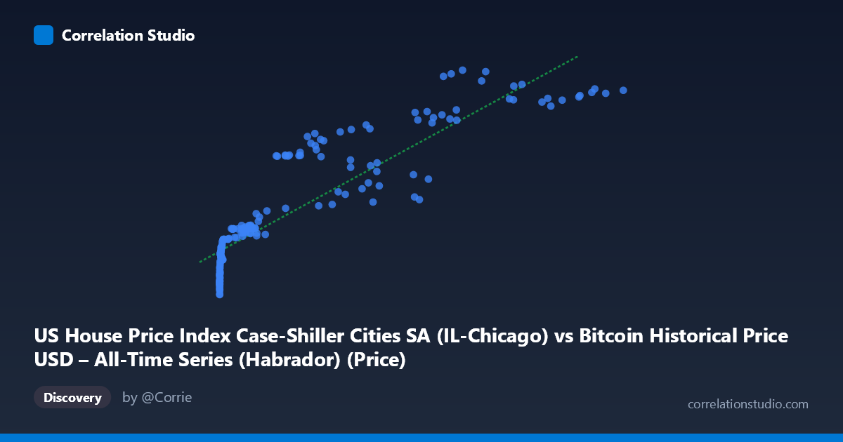
US House Price Index Case-Shiller Cities SA (IL-Chicago) vs Bitcoin Historical Price USD – All-Time Series (Habrador) (Price)
- Pearson correlation (r)
- 0.8962
- Spearman correlation
- 0.966
- p-value
- 0
- Sample size (n)
- 191
- 95% confidence interval
- 0.8642 to 0.921
- Granger causality
- None
- Granger optimal lag
- 2
- Time coverage
- 2010-08-01 to 2026-06-01
- Recomputed on refreshed data
- 2026-10-24 (r was 0.8929)
AI analysis
Analysis: Bitcoin Price vs. Chicago Case-Shiller Home Price Index
1. What the Visualization Reveals
The scatterplot shows a strongly monotonic, curved (logarithmic-like) relationship between Bitcoin's USD price (X-axis) and the Chicago Case-Shiller Home Price Index (Y-axis). Because Bitcoin's price spans nearly six orders of magnitude (from $0.06 to $118,670) while the home price index moves within a comparatively narrow band (107–227), the data is heavily compressed near the origin, with the vast majority of points clustered below X=10,000 and Y=145, and a sparser tail of high-Bitcoin-price observations extending the trend upward. The relationship visually resembles a logarithmic or power curve rather than a straight line, even though a linear model is reported.
2. Strength, Direction, and Statistical Confidence
The correlation is strong and positive (r = 0.891), with r² = 0.794 indicating that roughly 79% of the variance in the housing index can be statistically associated with Bitcoin's price level. The 95% CI [0.858, 0.918] is tight and does not cross zero, and the p-value of ~0 confirms this relationship is very unlikely due to chance. However, statistical significance here reflects shared temporal trend, not causal linkage — both series have risen dramatically over the 2010–2026 window, and the Granger causality tests confirm this: neither direction shows significant predictive power (Bitcoin→Housing: p=0.40; Housing→Bitcoin: p=0.22). This means past values of one series do not meaningfully improve forecasts of the other — the correlation is best interpreted as two independent upward trends coinciding in time, not one driving the other.
3. Notable Patterns and Features
- Non-linearity: The data show clear curvature — Y rises steeply at low X, then the rate of increase in Y slows as X grows into the tens of thousands, suggestive of a logarithmic relationship (log(X) vs Y would likely fit better than linear X vs Y). - Clustering: A dense cluster exists at very low Bitcoin prices (X < 1000) corresponding to Y values in the 107–140 range (roughly 2010–2013), and a second cluster at high Bitcoin prices (X 50,000) with Y in the 200–227 range (likely 2020s). - Sparse middle region: Mid-range Bitcoin prices ($1,000–$50,000) are less densely sampled, creating a somewhat "stretched" S-curve appearance. - No obvious outliers break the trend — the relationship, while non-linear, is remarkably smooth and consistent.
4. Confounding Factors and Caveats
This is a textbook case of spurious correlation via common time trend. Both series are non-stationary and generally trending upward over the same 15+ year period due to entirely different macroeconomic drivers: Bitcoin's price is influenced by adoption cycles, speculative demand, and crypto-specific events (halvings, exchange collapses, regulatory news), while the Case-Shiller index reflects mortgage rates, housing supply, wage growth, and regional Chicago market dynamics. Any two persistently trending time series — regardless of subject matter — will show high correlation without genuine causal connection. The lack of Granger causality strongly supports treating this as a coincidental trend alignment rather than a functional relationship. Additionally, the linear R² of 0.794 may be inflated by the extreme leverage of a handful of high-X outlier points (Bitcoin's parabolic price rises).
5. Actionable Insights and Further Investigation
- De-trend both series (e.g., using differencing, year-over-year % change, or detrending against a common macro variable like CPI) and re-test correlation; this will likely reveal much weaker or insignificant correlation once the shared time trend is removed. - Log-transform Bitcoin price before regression, given its multi-order-of-magnitude range — a log-linear model would likely fit better than the current linear specification and better reflect the visual curvature. - Avoid using this relationship for forecasting or trading strategies — the absence of Granger causality in either direction confirms neither series has predictive value for the other despite the high raw correlation. - Consider investigating shared underlying drivers (e.g., loose monetary policy, low interest rates, inflation expectations, or general risk-asset speculation) that may simultaneously inflate both Bitcoin and housing prices, which would be a more defensible causal story than a direct link between the two markets themselves.
X dataset: Bitcoin Historical Price USD – All-Time Series (Habrador)
Y dataset: US House Price Index Case-Shiller Cities SA
Part of experiment: Bitcoin - Bitcoin Historical Price USD – All-Time Series (Habrador) vs US House Price Index Case-Shiller Cities SA