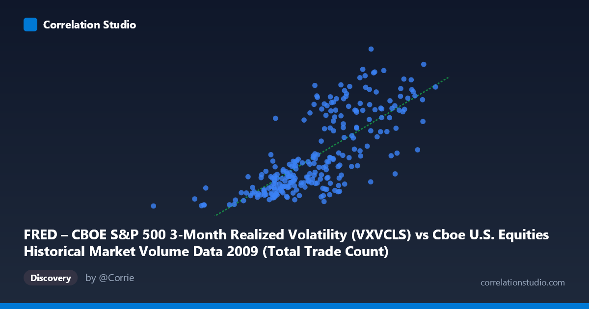
FRED – CBOE S&P 500 3-Month Realized Volatility (VXVCLS) vs Cboe U.S. Equities Historical Market Volume Data 2009 (Total Trade Count)
- Pearson correlation (r)
- 0.7416
- Spearman correlation
- 0.77
- p-value
- 0
- Sample size (n)
- 252
- 95% confidence interval
- 0.6803 to 0.7925
- Granger causality
- None
- Granger optimal lag
- 1
AI analysis
Scatterplot Analysis: CBOE S&P 500 3-Month Realized Volatility vs. Total Trade Count (2009)
Relationship Overview
The scatterplot reveals a moderately strong positive relationship between CBOE S&P 500 3-Month Realized Volatility (VXVCLS) and the Total Trade Count in U.S. equities markets across 2009. As realized volatility increases, trading activity (measured by total trade count) tends to rise correspondingly. This is intuitively consistent with market microstructure theory: elevated volatility typically prompts more frequent trading as investors rebalance, hedge, or capitalize on price dislocations. The linear regression equation (y = 9.87×10⁻⁶x + 6.61) confirms a positive slope, though the relatively small coefficient reflects the large scale difference between the X variable (spanning roughly 629K to 4.13M) and the Y variable (ranging ~22 to 55).
Correlation Strength and Statistical Framing
The Pearson correlation of r = 0.7416 indicates a meaningful positive association, but the more practically informative metric is r² = 0.5499, meaning that approximately 55% of the variance in realized volatility is explained by trade count (or vice versa). While substantial, this also means 45% of the variance remains unexplained, suggesting other important drivers are at work. The 95% confidence interval of [0.6803, 0.7925] is relatively tight given the sample size of n = 252, and the p-value of effectively zero confirms this relationship is not a statistical artifact. However, the Granger causality tests complicate the narrative significantly: neither direction (X→Y: F = 0.2237, p = 0.6366; Y→X: F = 0.0664, p = 0.7968) yields significant temporal predictive power at a 1-period lag. This means that while the two variables are clearly correlated contemporaneously, neither reliably leads the other in a predictive time-series sense — a critical distinction for any trading or forecasting application.
Patterns, Clusters, and Outliers
The sample points reveal several notable structural features. There appears to be a broad central cluster of observations in the X range of roughly 2.1M–3.1M paired with Y values of 24–35, suggesting a baseline regime of moderate volatility and typical trading volumes. A second, more dispersed upper cluster emerges around X values of 2.9M–4.1M paired with Y values of 38–55, representing high-volatility, high-activity episodes likely associated with post-crisis turbulence in early 2009. The point at (629,671, 22.43) stands out as a clear low-end outlier, sitting far from the main distribution on both axes and potentially representing an anomalous low-volume, low-volatility trading day. Several points in the upper-right quadrant (e.g., 4,134,002 / 47.03; 3,840,393 / 46.48) suggest that extreme trade counts are associated with the highest volatility readings, consistent with the market stress environment of early 2009.
Confounding Factors and Caveats
Several important caveats apply. First, 2009 was a highly atypical year — it encompassed the tail end of the global financial crisis and a subsequent recovery rally, meaning the volatility-volume relationship may have been amplified by crisis dynamics not representative of normal market conditions. Second, there is a dataset labeling asymmetry worth flagging: the X-axis is described as drawing from VXVCLS (the 3-month realized volatility index), while the Y-axis is labeled as "Total Trade Count" but sourced from the FRED CBOE dataset — this potential metadata mismatch warrants verification before drawing firm conclusions. Third, omitted variables such as VIX levels, macroeconomic news releases, Federal Reserve policy actions, and sector-specific shocks could be driving both variables simultaneously, inflating the apparent bivariate correlation. Finally, the absence of Granger causality at a 1-day lag does not rule out causality at longer lags or through nonlinear channels.
Actionable Insights and Further Investigation
Despite the non-significant Granger results, the strong contemporaneous correlation (r ≈ 0.74) suggests that trade count could serve as a useful real-time proxy for volatility regimes, even if it cannot predict future volatility. Practitioners building intraday risk models might incorporate trade count thresholds as a volatility regime indicator. For further investigation, it would be valuable to: (1) test Granger causality at lags beyond 1 period (e.g., 2–5 days) to rule out slower-moving predictive relationships; (2) segment the data by market phase (crisis period Q1 vs. recovery Q3–Q4) to test whether the correlation is regime-dependent; (3) add control variables such as VIX, bid-ask spreads, or institutional order flow to better isolate the volatility-volume mechanism; and (4) verify the axis dataset alignment to ensure the correct columns are being compared, given the noted discrepancy in dataset descriptions.
X dataset: Cboe U.S. Equities Historical Market Volume Data 2009
Y dataset: FRED – CBOE S&P 500 3-Month Realized Volatility
Part of experiment: Daily - Cboe U.S. Equities Historical Market Volume Data 2009 vs FRED – CBOE S&P 500 3-Month Realized Volatility