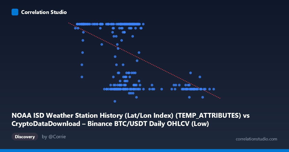
NOAA ISD Weather Station History (Lat/Lon Index) (TEMP_ATTRIBUTES) vs CryptoDataDownload – Binance BTC/USDT Daily OHLCV (Low)
- Pearson correlation (r)
- -0.4769
- Spearman correlation
- -0.3266
- p-value
- 0
- Sample size (n)
- 355
- 95% confidence interval
- -0.5535 to -0.3923
- Granger causality
- None
- Granger optimal lag
- 1
AI analysis
Analysis: BTC/USDT Trading Metric vs. Weather Station Index
1. What the Visualization Reveals
This scatterplot compares a column labeled as a NOAA weather station attribute (X-axis, ranging ~38,555–105,321) against a column labeled as BTC/USDT "Low" price data (Y-axis, ranging 5–24). The metadata is contradictory and appears mismatched — the X-axis values are far too large to be typical weather attributes (temperature, wind speed, etc.) and instead resemble BTC price data, while the Y-axis range (5–24) is inconsistent with realistic BTC/USDT low prices. This strongly suggests a column-label swap or misalignment in the dataset merge, and any economic or physical interpretation should be treated cautiously until the labeling is verified.
2. Strength, Direction, and Statistical Confidence
The correlation coefficient (r = -0.477) indicates a moderate negative relationship: as X increases, Y tends to decrease. However, r² = 0.2275 means only 22.75% of the variance in Y is explained by X — the majority (77%) of Y's variability is driven by other factors entirely. The 95% CI [-0.5535, -0.3923] is reasonably tight and excludes zero, and the p-value (~0) confirms this correlation is statistically significant and not due to chance, given the large sample size (n=355). That said, statistical significance here reflects sample size more than practical strength — this is a "real but weak-to-moderate" relationship. Critically, the Granger causality tests show no significant predictive direction in either direction (X→Y: p=0.657; Y→X: p=0.261), meaning neither variable helps forecast the other over time. This undermines any causal or lead-lag interpretation — the relationship is contemporaneous/associative at best, not predictive.
3. Notable Patterns and Clusters
The data shows a distinctive bimodal/banded structure rather than a smooth linear trend. A dense cluster sits at Y=24 across a wide X range (~41,000–70,000), suggesting a ceiling or saturation effect — possibly a capped/truncated value or a discrete category coded as "24." Separately, there's a cluster of low Y values (7–12) concentrated at higher X values (~60,000–98,000), and another low-Y cluster at lower X (~58,000–70,000). This creates a fan-like or two-regime pattern: one regime clusters at the Y-max regardless of X, while another regime shows more scattered, lower Y values as X increases. This is not consistent with a clean linear relationship — the linear fit (R²=0.227) is likely capturing an averaged trend across what may be two distinct subpopulations or a threshold effect rather than true linear covariance.
4. Confounding Factors and Caveats
Given the apparent label mismatch, the most important caveat is data provenance/integrity — verify which columns actually correspond to which dataset before drawing conclusions. If this genuinely mixes weather and crypto data joined by date, any correlation is likely spurious, driven by coincidental temporal alignment rather than a causal mechanism (classic confound in time-series merges). The apparent ceiling at Y=24 suggests possible data capping, binning, or an artificial maximum (e.g., hours in a day, a categorical code, or a data-quality artifact) that would violate assumptions of a continuous linear model. Seasonal patterns in both weather and BTC trading (e.g., annual cycles) could also produce a "correlation" purely through shared seasonality without any direct connection.
5. Recommendations for Further Investigation
1. Verify column mapping — confirm which physical/financial variables actually populate the X and Y axes before any further modeling. 2. Investigate the Y=24 cluster — determine if this is a legitimate value, a cap, or a data entry artifact; consider modeling this as a separate categorical regime. 3. Test non-linear or piecewise models — given the two-cluster pattern, a mixture model or segmented regression may fit better than a single linear line. 4. Control for time/seasonality — since both series may share seasonal cycles, test partial correlation controlling for date/month to rule out confounding. 5. Treat the relationship as associative, not predictive — given the null Granger causality results, avoid using one variable to forecast the other; explore other candidate predictors instead.
X dataset: CryptoDataDownload – Binance BTC/USDT Daily OHLCV
Y dataset: NOAA ISD Weather Station History (Lat/Lon Index)
Part of experiment: Bitcoin - CryptoDataDownload – Binance BTC/USDT Daily OHLCV vs NOAA ISD Weather Station History (Lat/Lon Index)