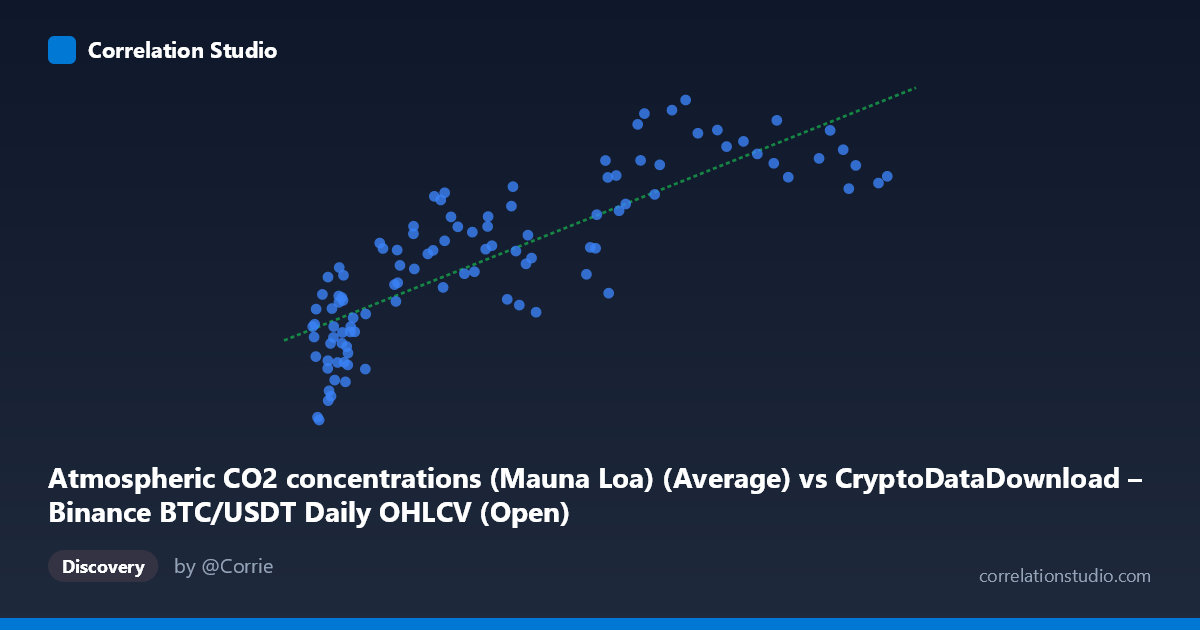
Atmospheric CO2 concentrations (Mauna Loa) (Average) vs CryptoDataDownload – Binance BTC/USDT Daily OHLCV (Open)
- Pearson correlation (r)
- 0.8274
- Spearman correlation
- 0.8616
- p-value
- 0
- Sample size (n)
- 106
- 95% confidence interval
- 0.756 to 0.8794
- Granger causality
- None
- Granger optimal lag
- 1
- Time coverage
- 2017-09-01 to 2026-06-01
- Recomputed on refreshed data
- 2026-10-08 (r was 0.8256)
AI analysis
Analysis: BTC/USDT Price vs. Atmospheric CO2 Concentration
1. What the Visualization Reveals
The scatterplot shows a strong positive association between Bitcoin's daily opening price and Mauna Loa atmospheric CO2 readings. As BTC price increases across its wide range (~$3,400 to ~$115,800), CO2 concentrations climb steadily from ~404 ppm to ~430 ppm. The relationship appears fairly monotonic and roughly linear in the lower-to-mid price range, with some flattening/plateauing behavior at higher BTC prices (above ~$60,000), where CO2 values cluster more tightly in the 419–427 ppm band despite large swings in price.
2. Strength, Direction, and Statistical Meaning
The correlation coefficient (r = 0.826) indicates a strong positive linear relationship, with r² = 0.682 meaning roughly 68% of the variance in CO2 readings can be statistically "explained" by BTC price movements. The 95% CI [0.752, 0.879] is reasonably tight and excludes zero, and the p-value (effectively 0) confirms this correlation is not due to random chance within this sample.
However, the Granger causality results are critical: neither variable predicts the other in a temporal/lead-lag sense (BTC→CO2: p=0.353; CO2→BTC: p=0.966). This strongly suggests the correlation is not causal in either direction — it's a classic case of two unrelated time series that both happen to trend upward over the same period (2017–2026), producing spurious correlation rather than genuine predictive relationship.
3. Notable Patterns and Features
- Non-linear saturation at high X: Above ~$60,000 BTC price, CO2 values compress into a narrower range (419–427 ppm) despite BTC ranging up to $115,000+, suggesting the linear model overstates the relationship at the extremes. - Low-X cluster: Many points cluster in the $3,000–$20,000 BTC range corresponding to CO2 in the 404–419 ppm range — this dense cluster (largely 2017–2020 data) heavily anchors the regression line. - Sparse high-X tail: Fewer points above $90,000 create leverage risk — a handful of observations may disproportionately influence the fitted slope. - No visible outliers that dramatically break the trend, but the compression at high values hints the true relationship may be logarithmic rather than linear.
4. Confounding Factors and Caveats
This is almost certainly a spurious correlation driven by shared trend/time. Both series are monotonically increasing over the 2017–2026 window for entirely unrelated reasons: BTC price reflects speculative market dynamics, adoption cycles, and macro liquidity conditions, while CO2 rises due to well-documented, independent anthropogenic emission trends. Any two non-stationary time series that trend in the same direction over a shared period will show inflated correlation — this is a textbook case for that statistical artifact. The Granger test results (no predictive causality) directly support this: there's no evidence of a real dynamic linkage between the systems.
5. Actionable Insights and Further Investigation
- Do not treat this correlation as meaningful for trading, forecasting, or policy. It should not inform any BTC price model or climate model. - De-trend both series (e.g., use first differences, or year-over-year change) and re-run the correlation. This would likely reveal the true (probably near-zero) relationship once the shared upward time trend is removed. - Check for unit-root/non-stationarity via ADF tests on both series — if both are non-stationary, standard Pearson correlation is inappropriate without cointegration testing. - If curious about genuine drivers, replace CO2 with variables plausibly linked to BTC (e.g., interest rates, USD index, mining hash rate, or on-chain metrics) for meaningful causal analysis. - This example is useful primarily as a pedagogical illustration of spurious correlation between unrelated trending time series.
X dataset: CryptoDataDownload – Binance BTC/USDT Daily OHLCV
Y dataset: Atmospheric CO2 concentrations (Mauna Loa)
Part of experiment: Bitcoin - CryptoDataDownload – Binance BTC/USDT Daily OHLCV vs Atmospheric CO2 concentrations (Mauna Loa)