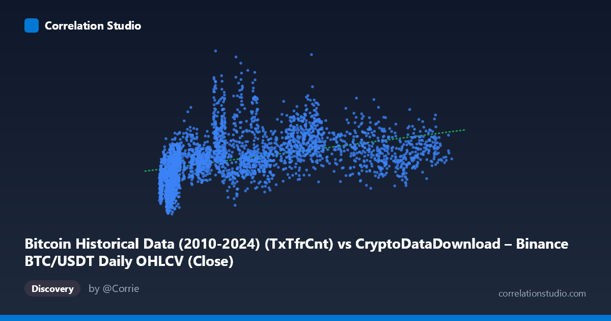
Bitcoin Historical Data (2010-2024) (TxTfrCnt) vs CryptoDataDownload – Binance BTC/USDT Daily OHLCV (Close)

Pearson correlation (r): 0.4347
Spearman correlation: 0.6016
p-value: 0
Sample size (n): 3191
95% confidence interval: 0.4061 to 0.4624
Granger causality: None
Granger optimal lag: 10
Time coverage: 2017-08-17 to 2026-05-20

AI analysis

Analysis: Bitcoin Transaction Count (TxTfrCnt) vs. BTC/USDT Closing Price

1. What the Visualization Reveals

The scatterplot shows a positive but noisy relationship between Bitcoin's daily transaction count and its closing price on Binance. Points are widely scattered rather than tightly clustered around the regression line (y = 2.51x + 718,413), indicating that transaction count is only a partial driver of price levels. The data spans nearly a decade (2017–2026), covering multiple market cycles (bull runs, crashes, and consolidation periods), which likely contributes to the dispersion since the same transaction count can correspond to very different price regimes depending on the broader market cycle.

2. Strength, Direction, and Statistical Confidence

The correlation coefficient (r = 0.4347) indicates a moderate positive relationship, but r² = 0.189 tells the more important story: only ~19% of the variance in price is explained by transaction count, leaving over 80% attributable to other factors. The 95% CI [0.406, 0.462] is fairly tight given the large sample (n=3,191), and the p-value of ~0 confirms the correlation is statistically significant and not due to chance — but statistical significance here reflects sample size more than practical predictive strength. Critically, the Granger causality test shows no significant predictive direction in either direction (X→Y: p=0.244; Y→X: p=0.924). This means neither variable reliably leads the other in time — the correlation is likely contemporaneous/structural (both driven by common underlying market conditions like adoption, speculation, or macro sentiment) rather than one causing or forecasting the other.

3. Notable Patterns and Non-Linear Features

Several observations suggest linearity is a poor fit: - Low-X, high-variance cluster: Many points with small X values (3,000–15,000 transactions) span a huge Y range (365K–1.68M price), suggesting price is highly volatile independent of low transaction activity — likely capturing quiet/bearish periods with wide price swings. - Compression at high X: Higher transaction counts (80,000) cluster more tightly in the 830K–1.05M price band, hinting at a possible saturation or ceiling effect rather than a continued linear increase. - The note that Spearman ρ exceeds Pearson r reinforces that the relationship is monotonic but non-linear — a log or power-law transformation of X (transaction count) may fit better, consistent with diminishing marginal price impact per additional transaction at scale.

4. Confounding Factors and Caveats

Several caveats limit causal interpretation: - Time-series autocorrelation: Both price and transaction count are trending/non-stationary series over 2017–2026; pooling all years together can create spurious correlation from shared long-term trends rather than a real functional relationship. - Omitted variables: Exchange volume, macroeconomic conditions, regulatory news, halving cycles, and speculative sentiment all plausibly drive both variables simultaneously, making transaction count a proxy rather than a cause. - Non-stationarity: Granger causality tests assume stationarity; if either series has unit roots (likely, given price trends), results should be interpreted cautiously — first-differencing or detrending is advisable before re-testing causality. - Scale mismatch: Transaction count is a blockchain-network metric while price is exchange-specific (Binance), so the two may not be as tightly coupled as on-chain price/activity pairs from a single source.

5. Actionable Insights and Further Investigation

- Do not use transaction count alone as a price predictor — the Granger test and low r² both argue against it having practical forecasting power. - Test non-linear models: fit log(X) vs Y or polynomial regression, given the Spearman/Pearson divergence, to see if r² improves meaningfully. - De-trend and test for stationarity (ADF test) before rerunning Granger causality; consider testing on returns/differences rather than levels to avoid spurious trend-driven correlation. - Segment by market regime (bull/bear/sideways) or halving cycle to check whether the X-Y relationship is stable over time or regime-dependent — pooling multiple cycles may be masking stronger localized relationships. - Incorporate additional covariates (active addresses, exchange volume, realized cap) in a multivariate model to isolate the marginal contribution of transaction count to price beyond shared trend effects.

X dataset: CryptoDataDownload – Binance BTC/USDT Daily OHLCV

Y dataset: Bitcoin Historical Data (2010-2024)

Part of experiment: Bitcoin - CryptoDataDownload – Binance BTC/USDT Daily OHLCV vs Bitcoin Historical Data (2010-2024)