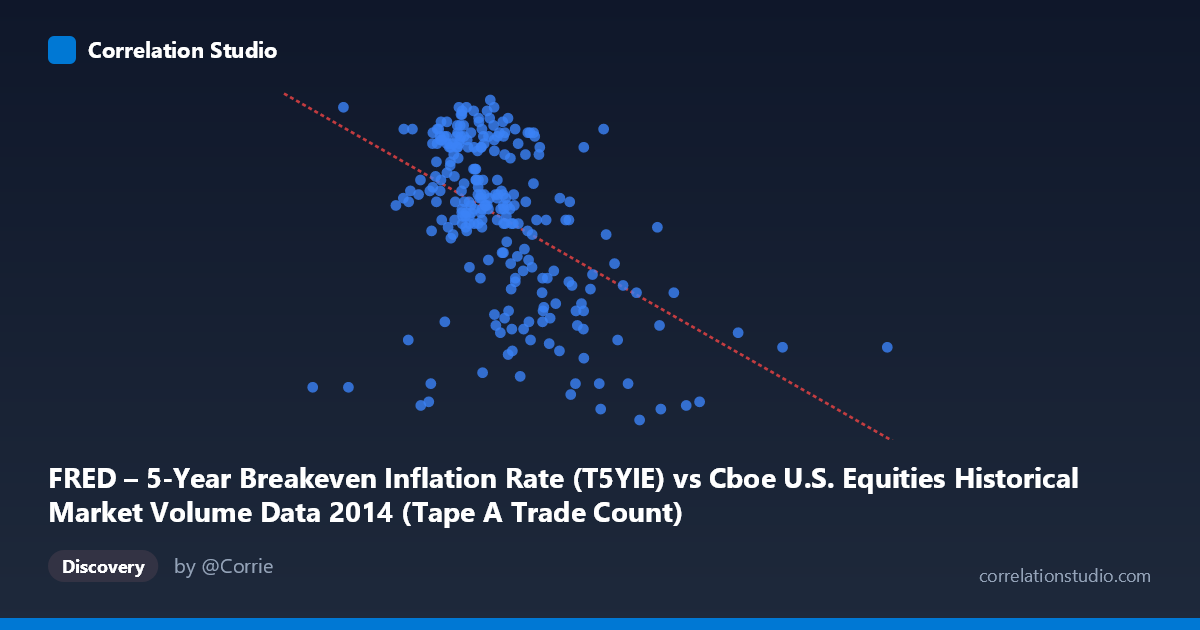
FRED – 5-Year Breakeven Inflation Rate (T5YIE) vs Cboe U.S. Equities Historical Market Volume Data 2014 (Tape A Trade Count)
- Pearson correlation (r)
- -0.4789
- Spearman correlation
- -0.4722
- p-value
- 0
- Sample size (n)
- 250
- 95% confidence interval
- -0.5692 to -0.3773
- Granger causality
- None
- Granger optimal lag
- 1
AI analysis
Analysis: 5-Year Breakeven Inflation Rate vs. Cboe U.S. Equities Tape A Trade Count (2014)
Relationship Overview
The scatterplot reveals a moderate negative relationship between U.S. equity market trading volume (Tape A trade count) and the 5-year breakeven inflation rate across 2014. As trade counts increase, the breakeven inflation rate tends to decline, and vice versa. The linear regression equation (y = -4.49×10⁻⁷x + 2.26) confirms this inverse slope, suggesting that higher equity market activity is associated with lower near-term inflation expectations. This is an intriguing pairing that likely reflects shared sensitivity to broader macroeconomic conditions rather than a direct causal mechanism between the two variables.
Correlation Strength and Statistical Significance
The Pearson correlation of r = -0.479 indicates a moderate negative association. The r² of 0.229 means that roughly 23% of the variance in the breakeven inflation rate is statistically accounted for by trade count — meaningful, but leaving approximately 77% of variation unexplained by this relationship alone. The 95% confidence interval of [-0.569, -0.377] is reasonably tight and does not cross zero, lending credibility to the direction of the effect. The p-value of 8.88×10⁻¹⁶ is extraordinarily small, confirming that this correlation is highly unlikely to be a chance artifact given the sample of 250 paired observations drawn from a population of 3,686 trading days. However, the Granger causality results are telling: neither direction (X→Y nor Y→X) achieves significance (F = 0.16, p = 0.69; F = 0.02, p = 0.88), meaning that neither variable temporally predicts the other at a one-period lag. This firmly cautions against any causal or predictive interpretation — the correlation is contemporaneous and likely co-driven by external factors.
Patterns, Clusters, and Outliers
The scatterplot shows considerable dispersion across the X-axis, with trade counts ranging from roughly 527,000 to over 2.5 million — a nearly fivefold spread. The bulk of observations cluster between approximately 900,000 and 1,400,000 trades, with the breakeven rate concentrated between 1.7 and 2.05 in that range, forming a relatively dense central cloud. Notable outliers exist at the high end of the X-axis — points near 2,171,000 and 2,537,988 trades correspond to breakeven rates of only 1.37, dragging the regression line downward and likely exerting disproportionate leverage on the correlation coefficient. There are also interesting low-X outliers (e.g., ~634,000 trades paired with a rate of 2.03), suggesting that very low-volume days coincided with elevated inflation expectations. A mild non-linear pattern may be present, where the negative relationship is strongest at the extremes and more diffuse in the middle range — a pattern worth testing with polynomial or spline regression.
Confounding Factors and Caveats
Several confounding dynamics complicate interpretation. Risk-off episodes — such as geopolitical shocks, Federal Reserve communications, or financial stress events in 2014 (e.g., Ukraine crisis, oil price collapse in H2 2014) — would simultaneously suppress inflation expectations and spike trading volume, creating the observed negative correlation without any direct link between the variables. Conversely, calm, low-volatility days tend to produce lower volume and stable-to-higher inflation expectations. Seasonality is also a concern: year-end and holiday periods distort both trade counts and market pricing. Additionally, the axis labels appear swapped in the dataset descriptions (Tape A Trade Count is labeled as a Y-axis variable from the FRED dataset, and vice versa), which warrants verification of the data pipeline before drawing firm conclusions. Finally, the Granger test uses only a lag of 1 period, and longer lags may reveal delayed dynamics not captured here.
Actionable Insights and Further Investigation
Given the absence of Granger causality, this relationship is best treated as a coincident indicator rather than a predictive one. Analysts should investigate volatility indices (VIX) or credit spreads as potential common drivers that explain both elevated trading activity and compressed inflation expectations simultaneously. Segmenting the 2014 data by macro regime (pre- and post-oil price shock in mid-2014) would likely reveal structural breaks in this correlation. It would also be valuable to test whether other inflation measures (e.g., 10-year breakeven, CPI surprises) show stronger or different correlations with trade volume. Finally, expanding the time series beyond 2014 would clarify whether this negative correlation is a persistent feature or an artifact of one unusual year characterized by notable deflationary pressures and episodic volatility spikes.
X dataset: Cboe U.S. Equities Historical Market Volume Data 2014
Y dataset: FRED – 5-Year Breakeven Inflation Rate
Part of experiment: Daily - Cboe U.S. Equities Historical Market Volume Data 2014 vs FRED – 5-Year Breakeven Inflation Rate