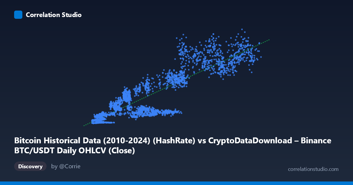
Bitcoin Historical Data (2010-2024) (HashRate) vs CryptoDataDownload – Binance BTC/USDT Daily OHLCV (Close)

Pearson correlation (r): 0.8909
Spearman correlation: 0.8817
p-value: 0
Sample size (n): 3191
95% confidence interval: 0.8835 to 0.8978
Granger causality: None
Granger optimal lag: 10
Time coverage: 2017-08-17 to 2026-05-20

AI analysis

Analysis of Bitcoin Hash Rate vs. Price Correlation

1. What the Visualization Reveals

The scatterplot shows a strong positive relationship between Bitcoin's network hash rate (X-axis) and its closing price (Y-axis). As hash rate increases from roughly 3,000 to 125,000 (units implied, likely EH/s or similar), price climbs from single-digit millions to over $1.3 billion in this dataset's scale—though the extreme Y-values suggest this may represent market cap or a scaled price metric rather than raw USD price. The overall shape is consistent with a positive linear trend, though the data shows considerable scatter, especially at higher hash rate values, indicating the relationship is not perfectly deterministic.

2. Strength, Direction, and Statistical Meaning

The correlation coefficient (r = 0.891) indicates a strong positive linear relationship, with r² = 0.794 meaning approximately 79% of the variance in Y is statistically explained by X. This is a substantial but not complete explanatory relationship—roughly 21% of price variance is driven by other factors entirely independent of hash rate. The tight 95% confidence interval [0.884, 0.898] combined with a p-value of ~0 confirms this correlation is highly statistically robust and not a product of sampling noise, given the large sample size (n=3,191).

However, the Granger causality results are critical context: neither variable significantly predicts the other in a temporal/lagged sense (X→Y: p=0.49; Y→X: p=0.165). This means that despite the strong contemporaneous correlation, historical hash rate values do not reliably forecast future price movements, and vice versa. This is an important distinction—correlation here should not be interpreted as one variable driving the other in a lead-lag sense. Both series likely respond to a common underlying driver (see confounders below) rather than one causing the other with a predictive lag structure.

3. Notable Patterns and Outliers

Examining the sample points, there's evident heteroscedasticity: variance in Y increases substantially as X increases. At low hash rates (~4,000-10,000), prices cluster tightly in the tens of millions. At higher hash rates (~60,000-110,000), price values scatter widely between 500 million and 1.3 billion, suggesting the relationship may not be strictly linear—a power-law or exponential relationship could fit better than the linear model provided. Notable "outlier-like" behavior appears in points like (58,746, 158M) and (54,884, 149M), which sit well below other points with similar hash rates (e.g., 61,806 → 515M), suggesting periods where price decoupled from hash rate growth—possibly bear market phases where miners continued operating/expanding infrastructure despite falling prices.

4. Confounders and Caveats

Both hash rate and price are likely driven by a common third factor: overall market cycle sentiment, halving events, and mining profitability expectations. Critically, hash rate itself is partly endogenous to price—rising prices incentivize more mining investment (new ASICs, capacity expansion), which mechanically raises hash rate with a lag, while crashing prices can trigger miner capitulation. This bidirectional economic linkage, occurring at irregular and evolving lags (network difficulty adjustments, hardware deployment timelines), likely explains why the Granger test shows no clean predictive direction—the true causal structure may involve variable, non-constant lags that violate the linear VAR assumptions Granger tests rely on. Additionally, both series are non-stationary trending time series (both grew substantially 2017-2024), which can produce spurious high correlation—this should be tested via cointegration analysis, not just Pearson r.

5. Suggested Further Investigation

Given the non-stationarity concern, I'd recommend: (a) testing both series for stationarity (ADF test) and running a cointegration test (Engle-Granger or Johansen) to determine if this is a genuine long-run equilibrium relationship rather than spurious trend correlation; (b) log-transforming both variables before regression, since the heteroscedastic fan-shaped scatter and multiplicative growth patterns suggest a log-log power law may fit better than the linear model (R² may improve); (c) segmenting the data by market regime (bull/bear/halving cycles) to see if the r² and slope are stable or regime-dependent; and (d) exploring alternative lag structures or nonlinear Granger causality (e.g., using difficulty-adjusted hash rate growth rates rather than levels) to properly capture the miner-investment feedback loop.

X dataset: CryptoDataDownload – Binance BTC/USDT Daily OHLCV

Y dataset: Bitcoin Historical Data (2010-2024)

Part of experiment: Bitcoin - CryptoDataDownload – Binance BTC/USDT Daily OHLCV vs Bitcoin Historical Data (2010-2024)