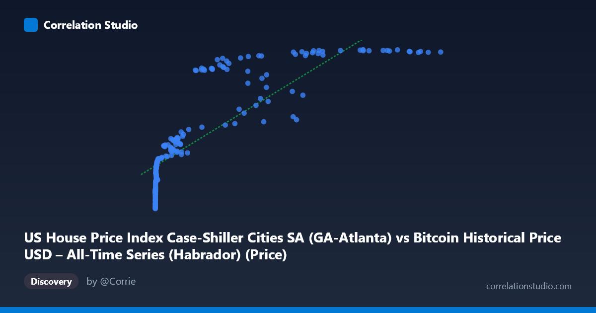
US House Price Index Case-Shiller Cities SA (GA-Atlanta) vs Bitcoin Historical Price USD – All-Time Series (Habrador) (Price)
- Pearson correlation (r)
- 0.8343
- Spearman correlation
- 0.965
- p-value
- 0
- Sample size (n)
- 187
- 95% confidence interval
- 0.7847 to 0.8732
- Granger causality
- None
- Granger optimal lag
- 1
AI analysis
Analysis: Bitcoin Price vs. US Housing Index (Atlanta Case-Shiller)
1. What the Visualization Reveals
The scatterplot shows a strong positive association between Bitcoin's historical USD price and the Atlanta Case-Shiller Home Price Index, but the relationship is clearly non-linear. At low Bitcoin prices (under ~$1,000), the housing index compresses tightly into a narrow band (85–140), while Bitcoin values span several orders of magnitude ($0.06 to ~$1,400). As Bitcoin prices climb past $10,000–$100,000+, the housing index rises but plateaus in a much narrower range (roughly 220–250), producing a curve that resembles a logarithmic or saturating S-shape rather than a straight line. This is a classic signature of two time series that are both trending upward over the same calendar period rather than mechanically driving one another.
2. Strength, Direction, and Uncertainty
The Pearson correlation (r = 0.834, r² = 0.696) indicates a strong positive linear relationship, with roughly 70% of the variance in one variable "explained" by the other in a naive linear sense. The 95% CI [0.785, 0.873] is tight and the p-value is effectively 0, meaning the correlation is highly unlikely to be a sampling artifact. However, statistical significance here should not be conflated with causal or mechanistic linkage — with n=187 paired points drawn from strongly trending series, high correlation is almost guaranteed. Critically, the Granger causality tests show no significant predictive direction in either direction (X→Y: p=0.294; Y→X: p=0.115). This is important: neither Bitcoin price changes reliably precede housing index changes, nor vice versa, at the tested lag. This strongly suggests the correlation is driven by a shared time trend (both assets appreciated over the 2010–2026 window) rather than one market causally influencing the other.
3. Notable Patterns and Outliers
Several features stand out: - Compression at both ends: many early Bitcoin observations (X < 100) cluster around Y ≈ 85–105, while many late/high-price observations (X 50,000) cluster around Y ≈ 245–250 — the housing index appears to be hitting a ceiling in this sample window. - Non-monotonic wobbles: points like (45092.81, 175.63) and (56973.18, 207.21) and (29111.52, 172.21) sit noticeably below the general trend for their X range, likely corresponding to Bitcoin bear-market or crash periods (e.g., 2018, 2022) where BTC price dropped while housing kept appreciating — a visible decoupling. - Logarithmic shape: the note that Spearman ρ exceeds Pearson r confirms monotonicity is stronger than linearity — a log-transform of X (or a saturating/logistic model) would likely fit far better than the linear model (R²=0.696).
4. Confounding Factors and Caveats
The most significant confound is shared temporal trend / spurious regression: both series generally rose over 2010–2026 due to independent macro forces (crypto adoption/speculation for Bitcoin; low interest rates, post-pandemic demand, and monetary policy for housing). Neither is likely a direct driver of the other. Additional caveats: Bitcoin's extreme scale (spanning 6+ orders of magnitude) means the linear fit is dominated by a few large-X points; the housing index is monthly and smoothed/seasonally adjusted while Bitcoin data is likely daily/higher-frequency, creating a temporal-resolution mismatch; and macro variables like inflation, USD strength, and Fed policy plausibly affect both assets simultaneously (a classic omitted-variable/confounder scenario).
5. Suggestions for Further Investigation
- Re-fit using log(X) or a log-log model given the non-linear shape and Spearman/Pearson discrepancy — likely to substantially improve fit. - Test for cointegration (e.g., Engle-Granger or Johansen test) rather than relying on levels correlation, since both series appear non-stationary/trending. - Introduce a common macro control (e.g., CPI, M2 money supply, or a time trend) and examine the partial correlation or use first-differenced/returns data instead of levels to assess whether the relationship holds after detrending. - Since Granger causality is insignificant, avoid framing this as predictive; instead treat it as a co-movement/diversification question relevant to portfolio construction rather than a lead-lag trading signal.
X dataset: Bitcoin Historical Price USD – All-Time Series (Habrador)
Y dataset: US House Price Index Case-Shiller Cities SA
Part of experiment: Bitcoin - Bitcoin Historical Price USD – All-Time Series (Habrador) vs US House Price Index Case-Shiller Cities SA