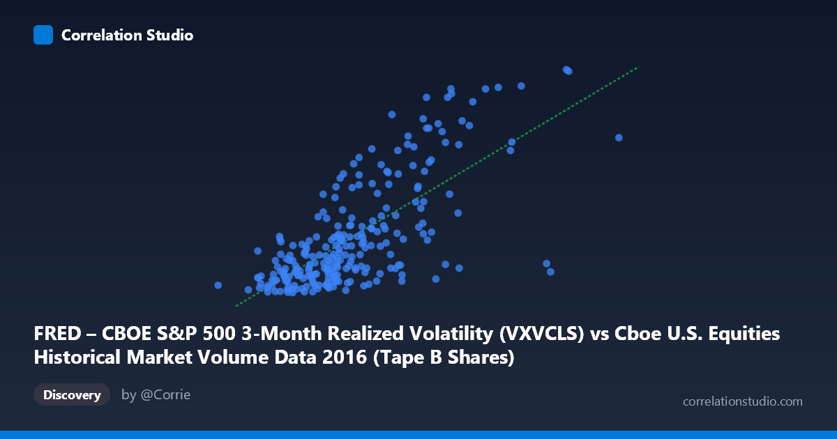
FRED – CBOE S&P 500 3-Month Realized Volatility (VXVCLS) vs Cboe U.S. Equities Historical Market Volume Data 2016 (Tape B Shares)
- Pearson correlation (r)
- 0.7116
- Spearman correlation
- 0.6745
- p-value
- 0
- Sample size (n)
- 252
- 95% confidence interval
- 0.6447 to 0.7677
- Granger causality
- None
- Granger optimal lag
- 1
- Time coverage
- 2016-01-04 to 2016-12-30
- Recomputed on refreshed data
- 2026-10-22 (r was 0.7116)
AI analysis
Analysis: CBOE S&P 500 3-Month Realized Volatility vs. Tape B Shares Volume (2016)
Relationship Overview The scatterplot reveals a moderately strong positive relationship between CBOE S&P 500 3-Month Realized Volatility (VXVCLS) and Tape B share volume in U.S. equity markets during 2016. As volatility increases, Tape B trading volume rises correspondingly, which aligns with the well-established market intuition that heightened uncertainty drives greater trading activity. The linear regression equation (y = 7.14×10⁻⁸x + 10.60) confirms this positive slope, suggesting that for every ~14 million additional shares of Tape B volume, realized volatility increases by approximately one index point. The relationship is visible across a wide range of volume values, from roughly 43.5M to 233.9M shares, with the bulk of observations clustering in the 75M–130M range paired with volatility readings between 15 and 20.
Correlation Strength and Statistical Significance The correlation coefficient of r = 0.712 indicates a moderately strong positive association, and critically, the R² of 0.506 means that approximately 50.6% of the variance in realized volatility is explained by Tape B volume alone — a meaningful but incomplete picture. The 95% confidence interval for r spans [0.645, 0.768], a relatively tight band that reflects the reasonably large paired sample (n = 252), and the p-value of effectively zero confirms this is not a chance finding. However, the Granger causality tests tell a more cautionary tale: neither direction (X→Y nor Y→X) achieves significance (F = 0.005, p = 0.944 and F = 0.243, p = 0.623, respectively). This means that while the two variables move together contemporaneously, neither reliably predicts the other's future values at a one-period lag — correlation here is synchronous, not predictive.
Patterns, Clusters, and Outliers The data exhibits several notable structural features. The bulk of observations form a dense central cluster around the mean (107M shares, volatility ~18), suggesting a stable baseline regime for most of 2016. However, there is a clear upper-right outlier cluster — points near (170M shares, 26.7) and (233M shares, 27.8) — that likely corresponds to episodic risk events such as the Brexit vote in late June or post-U.S. election turbulence in November. These high-leverage points disproportionately influence the regression slope and correlation magnitude. There also appears to be a lower-left sparse region with very low volume and low volatility (sub-16), suggesting a quiet-market regime. The relationship may not be strictly linear; the upper tail fans out, hinting at a potential heteroscedastic or curved relationship where volatility amplifies non-linearly during extreme volume episodes.
Confounding Factors and Caveats Several important caveats limit straightforward interpretation. First, Tape B captures only a subset of U.S. equity volume (NYSE American and regional exchanges), so using it as a proxy for total market activity introduces selection bias. Second, the axis labels appear to be swapped in the metadata — X is described as VXVCLS yet labeled from the Cboe volume dataset, and Y draws from FRED volatility data — warranting verification before drawing firm conclusions. Third, shared macro drivers (e.g., Federal Reserve announcements, geopolitical shocks) almost certainly act as common confounders, simultaneously elevating both volatility and volume without one directly causing the other. Fourth, the population size of N = 3,622 versus a sample of n = 252 raises questions about sampling representativeness, particularly if the sampled days over- or under-represent high-volatility episodes.
Actionable Insights and Further Investigation Practitioners should be cautious about using this relationship for short-term forecasting given the failed Granger causality tests — knowing today's volume does not significantly improve predictions of tomorrow's volatility, and vice versa. More productive next steps would include: (1) testing non-linear models (e.g., log-log or polynomial regression) to better capture the upper-tail behavior; (2) incorporating total consolidated tape volume (Tapes A, B, and C combined) to assess whether the relationship strengthens; (3) segmenting the analysis by market regime (pre/post-Brexit, pre/post-election) to test whether the correlation is event-driven rather than structural; and (4) introducing control variables such as VIX levels, Federal Reserve policy dates, or market breadth indicators to isolate the independent contribution of volume to volatility. The ~49% of unexplained variance represents a substantial opportunity for model enrichment.
X dataset: Cboe U.S. Equities Historical Market Volume Data 2016
Y dataset: FRED – CBOE S&P 500 3-Month Realized Volatility
Part of experiment: Daily - Cboe U.S. Equities Historical Market Volume Data 2016 vs FRED – CBOE S&P 500 3-Month Realized Volatility