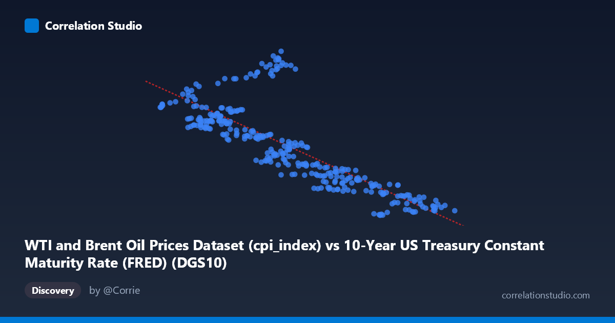
WTI and Brent Oil Prices Dataset (cpi_index) vs 10-Year US Treasury Constant Maturity Rate (FRED) (DGS10)
- Pearson correlation (r)
- -0.8017
- Spearman correlation
- -0.8587
- p-value
- 0
- Sample size (n)
- 306
- 95% confidence interval
- -0.8384 to -0.7577
- Granger causality
- None
- Granger optimal lag
- 1
AI analysis
Analysis: 10-Year Treasury Yield vs. Real WTI Crude Oil Prices (1986–2026)
1. Overall Relationship The scatterplot reveals a clear negative relationship between the 10-year US Treasury constant maturity yield (X-axis) and real (CPI-adjusted) WTI crude oil prices (Y-axis). As Treasury yields rise, real oil prices tend to fall, and vice versa. The linear regression equation (y = −20.23x + 295.09) quantifies this: each one-percentage-point increase in the 10-year yield is associated with approximately a $20 decline in real oil prices. The data span four decades (1986–2026), covering multiple economic cycles, making this a structurally meaningful — if complex — relationship rather than a short-term artifact.
2. Correlation Strength, Explained Variance, and Causality The correlation coefficient of r = −0.80 indicates a strong negative linear association. The R² of 0.643 means that roughly 64% of the variance in real oil prices is explained by Treasury yields in this sample — a substantial share for a two-variable relationship in macroeconomic data, though it also means 36% of the variance remains unexplained by yields alone. The 95% confidence interval for r of [−0.838, −0.758] is relatively tight and lies entirely in negative territory, and the p-value of effectively zero confirms this is not a chance finding across n = 306 paired observations. However, the Granger causality results are critical here: neither direction clears conventional significance thresholds (X→Y: F = 3.67, p = 0.057; Y→X: F = 0.72, p = 0.397). The X→Y direction is borderline suggestive but falls just short at the 5% level, and Y→X shows no predictive power at all. This means neither variable reliably predicts the other in a temporal, lagged sense — the correlation reflects a co-movement likely driven by shared macro forces rather than a direct causal channel.
3. Patterns, Clusters, and Notable Features Several structural features are visible in the sample points. There is a high-yield, low-oil-price cluster (yields ~7–9%, oil ~115–170) consistent with the early 1990s and potentially late 1980s, when real rates were elevated and oil was relatively cheap in inflation-adjusted terms. Conversely, a low-yield, high-oil-price cluster (yields ~1–3%, oil ~220–315) reflects the post-2008 and post-2020 era of near-zero interest rates coinciding with oil price spikes. There are notable outliers with high dispersion at mid-range yields (~3–5%), where oil prices range widely from ~160 to over 315 — suggesting this zone captures multiple distinct regimes (e.g., the mid-2000s commodity boom vs. more recent cycles). The relationship appears broadly linear but with heteroscedastic spread, widening at lower yields, which may indicate a non-linear or regime-dependent dynamic at the extremes.
4. Confounding Factors and Interpretation Caveats This correlation almost certainly reflects common causation by broader macroeconomic cycles rather than a direct mechanical link. Several confounders are worth flagging: (a) Federal Reserve policy simultaneously drives both Treasury yields and economic demand (which affects oil consumption); (b) inflation regimes — since oil prices here are CPI-adjusted and CPI itself affects Treasury yields via Fed reaction functions, there may be a constructed co-movement artifact; (c) global supply shocks (OPEC decisions, geopolitical disruptions) can spike oil prices independently of yield environments; and (d) secular trends — both variables have undergone long-run structural shifts over 40 years (the "Great Moderation," the zero-lower-bound era, post-COVID inflation), meaning the dataset may be pooling fundamentally different regimes. The borderline Granger p-value (0.057) also warrants caution — it could reflect a weak lagged signal or simply model mis-specification at lag = 1.
5. Actionable Insights and Further Investigation For practitioners, this relationship suggests Treasury yield environments should be incorporated into oil price forecasting models, but not as a standalone predictor given the 36% unexplained variance and lack of confirmed Granger causality. Several next steps would sharpen the analysis: (1) Regime-segmented analysis — split the data into distinct monetary policy eras (pre-/post-2008, post-COVID) to test whether the correlation is stable or driven by one period; (2) Multiple regression incorporating inflation expectations (TIPS spreads), USD index, and global demand proxies to isolate the independent yield effect; (3) Test longer Granger lags (3–12 periods) since monthly or quarterly transmission mechanisms may operate on longer horizons than lag = 1; (4) Examine non-linear models (piecewise regression or GAMs) given the visible heteroscedasticity at low yields; and (5) Consider cointegration testing (Engle-Granger or Johansen) to determine whether these two series share a long-run equilibrium, which would be more meaningful than short-lag Granger tests for data spanning 40 years.
X dataset: 10-Year US Treasury Constant Maturity Rate (FRED)
Y dataset: WTI and Brent Oil Prices Dataset
Part of experiment: Daily - 10-Year US Treasury Constant Maturity Rate (FRED) vs WTI and Brent Oil Prices Dataset