Bitcoin Historical Data (2010-2024) (AdrActCnt) vs Bitcoin Historical Price USD – All-Time Series (Habrador) (Price)
- Pearson correlation (r)
- 0.4927
- Spearman correlation
- 0.8211
- p-value
- 0
- Sample size (n)
- 5764
- 95% confidence interval
- 0.4729 to 0.512
- Granger causality
- None
- Granger optimal lag
- 10
AI analysis
Analysis: Bitcoin Active Address Count vs. Price
1. Overview of the Relationship
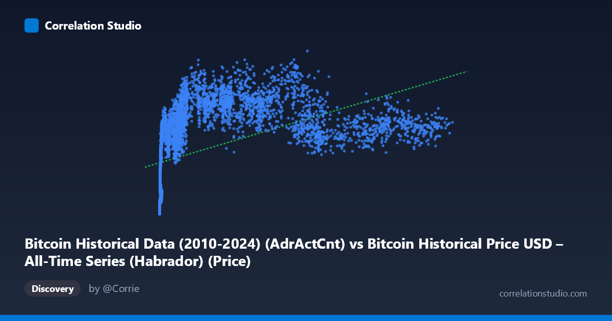
The scatterplot depicts Bitcoin's daily active address count (X) against its USD price (Y) across nearly the entire trading history (2010–2026). The data reveals a positive but noticeably non-linear relationship: at low active-address counts (under ~1,000), prices cluster tightly at low values (hundreds to low thousands of dollars), consistent with Bitcoin's early years. As active addresses scale into the tens of thousands, price shows much greater dispersion — ranging from roughly $500,000 to over $1,300,000 for similar X values in the 20,000–90,000 range. This fanning-out pattern is a hallmark of a relationship that saturates or decouples at higher levels of network activity.
2. Strength, Direction, and Statistical Confidence
The Pearson correlation (r = 0.493) indicates a moderate positive linear association, with r² = 0.243 meaning only about 24% of the variance in price is explained by active address count in a linear framework. The 95% CI [0.473, 0.512] is narrow, and the p-value is effectively zero — so despite the modest effect size, we can be highly confident the true correlation is non-zero and reliably positive; this is a function of the large sample (n = 5,764) rather than evidence of a tight relationship. Critically, the Granger causality tests show no significant predictive direction in either direction (X→Y p = 0.934, Y→X p = 0.422) at the optimal lag of 10 periods. This means neither variable reliably forecasts future movements in the other over time — the contemporaneous correlation does not translate into temporal lead/lag predictability, which is an important distinction from causal influence.
3. Notable Patterns and Non-linearity
The regression line (y = 5.92x + 429,086) is a poor descriptor of the underlying structure. The note that Spearman ρ exceeds Pearson r confirms a monotonic-but-curved relationship is more appropriate — likely logarithmic or power-law in X, which aligns with typical network-adoption dynamics (diminishing marginal price impact per additional active address). Visually, low-X points near the origin (X < 20, Y < 50,000) represent Bitcoin's earliest history and are tightly bunched, while the high-X region (50,000–125,000) is characterized by wide vertical scatter, indicating price is driven by other factors once the network matures. There also appear to be several "plateaus" or clusters (e.g., clusters around X≈40,000–65,000 with Y ranging widely from $600K to $1.26M), suggesting distinct market regimes/cycles rather than one continuous function.
4. Confounders and Caveats
This is time-series data, so both variables are likely non-stationary and trending upward over the sample period, which can inflate correlation due to shared time trends rather than genuine dependency (spurious correlation risk). Bitcoin price is influenced by many exogenous factors not captured here — macroeconomic conditions, regulatory news, exchange liquidity, halving cycles, speculative sentiment, and derivatives market activity — any of which could be driving both price and address activity simultaneously (confounding by market cycle phase). Additionally, active address count can be inflated by non-economic activity (e.g., wallet-shuffling, exchange internal transfers, or dust attacks), weakening its role as a pure "usage" proxy.
5. Recommendations for Further Investigation
Given the evident non-linearity, refitting with log(X) or log(Y) transformations (or a power-law model) should substantially improve explanatory power over the current linear r². Since both series are time-indexed, testing for stationarity (ADF/KPSS) and considering first-differencing or cointegration analysis (e.g., Engle-Granger/Johansen) would clarify whether the relationship is spurious or reflects a genuine long-run equilibrium — despite the lack of Granger causality at lag 10, shorter lags or a VECM approach might reveal structure. Finally, segmenting the analysis by market cycle/era (early, 2017 bull run, 2020–21 bull run, post-2022 crash, etc.) would help determine if the relationship's strength and shape vary meaningfully by regime, which the current pooled analysis may be obscuring.
X dataset: Bitcoin Historical Price USD – All-Time Series (Habrador)
Y dataset: Bitcoin Historical Data (2010-2024)
Part of experiment: Bitcoin - Bitcoin Historical Price USD – All-Time Series (Habrador) vs Bitcoin Historical Data (2010-2024)