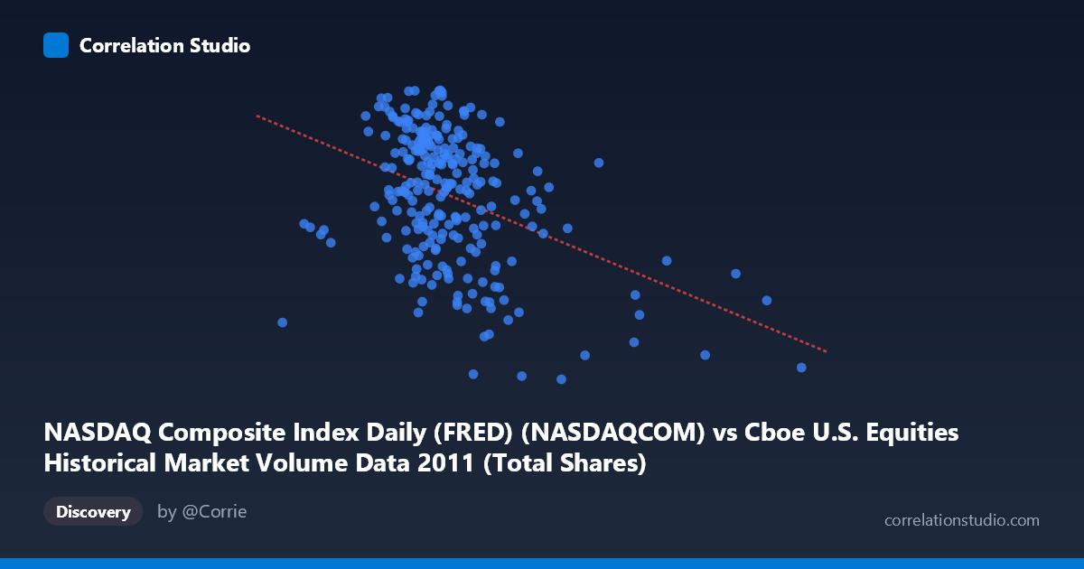
NASDAQ Composite Index Daily (FRED) (NASDAQCOM) vs Cboe U.S. Equities Historical Market Volume Data 2011 (Total Shares)
- Pearson correlation (r)
- -0.4005
- Spearman correlation
- -0.3329
- p-value
- 0
- Sample size (n)
- 252
- 95% confidence interval
- -0.4994 to -0.2913
- Granger causality
- None
- Granger optimal lag
- 10
AI analysis
Analysis: NASDAQ Composite Index vs. Cboe U.S. Equities Total Shares Volume (2011)
Relationship Overview The scatterplot reveals a modest negative relationship between the NASDAQ Composite Index level and total U.S. equities share volume traded on Cboe exchanges throughout 2011. As the NASDAQ index climbed higher, daily trading volume tended to decline — a counterintuitive pattern at first glance, but one consistent with well-documented market microstructure behavior where elevated uncertainty and volatility (typically at lower index levels) drives higher participation, while calmer bull-trending markets see reduced churn. The linear regression equation (y = -4.01×10⁻⁷x + 2887.1) quantifies this: each 1-billion-unit increase in volume is associated with a roughly 400-point decline in the index, though causation cannot be assumed.
Correlation Strength and Statistical Significance The Pearson correlation of r = -0.40 indicates a moderate negative association, but the coefficient of determination r² = 0.16 is the more sobering figure — NASDAQ index level explains only ~16% of the variance in daily share volume. The remaining 84% is attributable to factors entirely outside this model. The 95% confidence interval of [-0.499, -0.291] is meaningfully bounded away from zero, and the p-value of 3.99×10⁻¹¹ (with n = 252 paired observations from a population of 3,780) confirms this correlation is highly statistically significant — not a sampling artifact. However, statistical significance here is somewhat expected given the sample size; practical significance is limited. Critically, Granger causality testing finds no significant predictive direction in either direction (X→Y: F = 1.60, p = 0.107; Y→X: F = 0.51, p = 0.879), meaning neither variable reliably predicts the other across the tested lag structure of 10 periods. This rules out straightforward temporal lead-lag exploitation.
Notable Patterns, Clusters, and Outliers Several features stand out in the data. The bulk of observations cluster in the X range of ~400M–650M shares and Y range of ~2,550–2,850 index points, forming a loose but visible downward-sloping core. There are notable right-tail outliers at very high volume levels (approaching ~878M–1.2B shares) that correspond to lower index values, consistent with high-stress trading days — likely tied to the August 2011 U.S. debt ceiling crisis and S&P credit downgrade, which generated extreme volume spikes. Conversely, the low-volume, high-index quadrant (upper-left) is sparsely populated. The spread of Y values across similar X values is wide, reinforcing the weak explanatory power of the linear model and suggesting heteroscedasticity — variance in volume appears larger at lower index levels.
Confounding Factors and Caveats Several important caveats apply. First, 2011 was an atypical year marked by the European sovereign debt crisis, the August flash correction, and elevated macro volatility — making any single-year relationship potentially unrepresentative of long-run dynamics. Second, secular trends in both series (volume declining year-over-year due to market structure changes; index trending upward then crashing) could produce a spurious correlation driven by shared time trends rather than a direct mechanism. Third, the index level is not the same as returns or volatility — using VIX or realized volatility as the X variable might reveal a far stronger relationship. Finally, aggregating across all Cboe-affiliated venues may mask venue-specific routing behaviors that respond differently to market conditions.
Actionable Insights and Further Investigation Practitioners should not use NASDAQ index level alone as a volume forecasting input given the 84% unexplained variance and absence of Granger causality. More productive next steps include: (1) substituting realized volatility or VIX for index level to test whether fear-driven volume is the true underlying driver; (2) decomposing volume by trade size or venue to identify whether retail vs. institutional activity responds differently to index levels; (3) extending the time series beyond 2011 to test whether this negative correlation is stable or specific to this volatile year; and (4) applying a non-linear or regime-switching model to capture the apparent structural break between low-stress and high-stress market periods visible in the outlier cluster. The Granger results suggest any predictive model should incorporate exogenous macro variables rather than relying on cross-series lagged values.
X dataset: Cboe U.S. Equities Historical Market Volume Data 2011
Y dataset: NASDAQ Composite Index Daily (FRED)
Part of experiment: Daily - Cboe U.S. Equities Historical Market Volume Data 2011 vs NASDAQ Composite Index Daily (FRED)