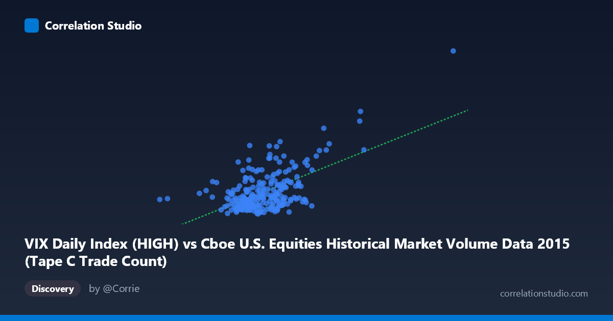
VIX Daily Index (HIGH) vs Cboe U.S. Equities Historical Market Volume Data 2015 (Tape C Trade Count)
- Pearson correlation (r)
- 0.5856
- Spearman correlation
- 0.3853
- p-value
- 0
- Sample size (n)
- 252
- 95% confidence interval
- 0.4981 to 0.6613
- Granger causality
- None
- Granger optimal lag
- 1
AI analysis
Analysis: VIX Daily Index (HIGH) vs. Tape C Trade Count
Overview of the Relationship
The scatterplot reveals a moderate positive relationship between the Cboe VIX Daily Index High values and Tape C Trade Count across U.S. equities exchanges in 2015. As VIX High readings increase, Tape C trade counts tend to rise as well, which is intuitively consistent with market microstructure theory: elevated volatility typically drives heightened trading activity as market participants respond to uncertainty, rebalance portfolios, and execute hedging strategies. The linear regression equation (y = 2.237e-05x + 0.844) reflects this upward slope, though the relationship is clearly not tight enough to be considered deterministic.
Correlation Strength and Statistical Significance
The Pearson correlation of r = 0.5856 indicates a moderate positive association, with r² = 0.3429 meaning that roughly 34.3% of the variance in Tape C Trade Count is explained by VIX High levels — leaving approximately 65.7% attributable to other factors. The 95% confidence interval of [0.4981, 0.6613] is reasonably narrow given the sample size of n = 252, and the p-value of effectively 0 confirms the correlation is highly statistically significant against the null hypothesis of no relationship. However, statistical significance should not be conflated with practical or causal significance. Critically, the Granger causality tests fail in both directions (X→Y: F = 0.3402, p = 0.5603; Y→X: F = 0.0350, p = 0.8518), meaning neither variable temporally predicts the other at the optimal 1-period lag. This strongly suggests the two variables are contemporaneously correlated — likely driven by shared underlying market forces — rather than one causing the other in a predictive sense.
Notable Patterns, Clusters, and Outliers
The sample data reveals several important structural features. The bulk of observations cluster in the lower-left region of the plot, with VIX High values concentrated in the 600,000–900,000 range and Tape C counts predominantly between 12 and 20, suggesting these represent typical low-to-moderate volatility trading days. There is a visible dispersion fan as X increases — variance in Y appears to expand at higher VIX levels, hinting at heteroscedasticity. Several notable outliers stand out: the point near (291,078; 15.88) sits far to the left of the distribution and may represent an anomalous or data-quality issue, while the point near (1,194,527; 38.06) and another near (1,611,853; 53.29) in the full range represent extreme high-volatility, high-trade-count events — likely corresponding to specific market stress episodes in 2015, such as the August flash crash.
Confounding Factors and Interpretive Caveats
Several important caveats apply. First, the axes appear to be swapped from standard convention — the dataset metadata indicates VIX (HIGH) is on the X-axis and Tape C Trade Count on the Y-axis, yet these originated from different datasets, raising the possibility of alignment or join artifacts. Second, the population size of N = 3,302 versus the paired sample of n = 252 suggests substantial data was excluded from the pairing, which could introduce selection bias. Third, day-of-week effects, scheduled economic announcements, expiration cycles, and seasonal patterns (e.g., August–September 2015 volatility spike) all independently affect both VIX and trade volumes, acting as common drivers that inflate the observed correlation without implying a direct mechanism. The lack of Granger causality further underscores that both variables likely respond simultaneously to external shocks rather than influencing each other.
Actionable Insights and Further Investigation
For practitioners, this correlation suggests that Tape C trade volume can serve as a rough contemporaneous signal of market stress alongside VIX, but should not be used as a predictive leading indicator in either direction. To deepen this analysis, it would be valuable to: (1) disaggregate by volatility regime (low: VIX < 15, moderate: 15–25, high: 25) to test whether the relationship is non-linear or regime-dependent; (2) test higher-order lags in Granger causality beyond lag-1 to rule out delayed predictive effects; (3) control for calendar effects and macroeconomic announcements to isolate the genuine volatility-volume relationship; and (4) apply a log transformation to both variables, as financial volume and volatility data typically exhibit right-skewed distributions where log-linear models often fit substantially better and reduce heteroscedasticity concerns.
X dataset: Cboe U.S. Equities Historical Market Volume Data 2015
Y dataset: VIX Daily Index
Part of experiment: Daily - Cboe U.S. Equities Historical Market Volume Data 2015 vs VIX Daily Index