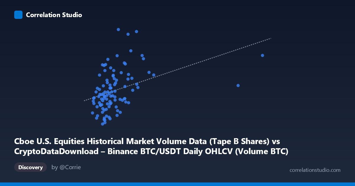
Cboe U.S. Equities Historical Market Volume Data (Tape B Shares) vs CryptoDataDownload – Binance BTC/USDT Daily OHLCV (Volume BTC)
- Pearson correlation (r)
- 0.3859
- Spearman correlation
- 0.464
- p-value
- 0.000052
- Sample size (n)
- 104
- 95% confidence interval
- 0.2088 to 0.5385
- Granger causality
- None
- Granger optimal lag
- 10
- Time coverage
- 2026-01-02 to 2026-06-25
- Recomputed on refreshed data
- 2026-10-23 (r was 0.3859)
AI analysis
Analysis: Cboe Equities Volume (Tape B) vs. Binance BTC/USDT Volume
1. Relationship Overview
The scatterplot shows a modest positive relationship between the two variables, with the vast majority of observations clustered in the lower-left region (X: 10,000–35,000; Y: 140M–320M) and a sparse tail of higher values extending outward. A handful of points—most notably one near X=106,298 and a few in the 35,000–45,000 range—sit well outside the main cluster, giving the scatter a somewhat "comet-shaped" distribution rather than a tight linear band. Within the dense cluster, the upward trend is visible but noisy, with substantial vertical scatter at any given X value.
2. Strength, Direction, and Statistical Confidence
The correlation coefficient (r = 0.4243) indicates a weak-to-moderate positive relationship. The r² of 0.18 means only 18% of the variance in Y is explained by X, leaving 82% attributable to other factors or noise. The 95% CI [0.24, 0.58] is fairly wide but excludes zero, and the p-value (3.08E-05) confirms the correlation is statistically significant and unlikely due to chance—but statistical significance here reflects a real, non-trivial association, not a strong predictive relationship. Critically, the Granger causality tests show no significant predictive direction in either direction (X→Y: p=0.756; Y→X: p=0.909). This means that despite the contemporaneous correlation, neither series helps forecast the other's future values based on past values—the relationship appears to be either coincidental, driven by a shared external factor, or purely contemporaneous rather than lead-lag in nature.
3. Notable Patterns and Outliers
Several features stand out: - High-leverage outlier: The point at X≈106,298, Y≈322.9M is far removed from the rest of the data and likely has outsized influence on the regression slope and r value. - Secondary cluster: A group of points in the X=28,000–45,000 range with notably high Y values (300M–390M) suggests a possible sub-population or regime where the relationship strengthens. - Dense core cluster: Most points sit in a "cloud" between X=10,000–25,000, where Y varies enormously (137M to 390M) with little apparent structure—suggesting X alone is a poor predictor in this range. - No strong evidence of nonlinearity (e.g., curvature) beyond what the outlier and secondary cluster introduce.
4. Confounding Factors and Caveats
Several caveats warrant attention: - Mismatched asset classes: Comparing Cboe equities volume (Tape B, traditional stocks) to Binance BTC/USDT volume conflates two very different markets with different drivers (macro equity flows vs. crypto-specific sentiment, regulation, leverage cycles). - Time aggregation mismatch: With only 90 paired points against 1,980 in the population and a ~4.5-month window (Jan–May 2026), the sample may not capture seasonal or regime effects adequately. - Outlier sensitivity: The extreme X value (106,298) is nearly 3x the next-highest X value and could be a data anomaly or a genuine market event (e.g., an equity volatility spike) that disproportionately affects the correlation estimate. - Common confounders: Both markets may be jointly influenced by macro factors (interest rate announcements, risk-on/risk-off sentiment, major news events) without any direct causal link between them.
5. Suggested Next Steps
- Remove/isolate the outlier (X≈106,298) and recompute r² to test result stability. - Investigate the secondary cluster (X=28,000–45,000) to determine if it corresponds to a specific date range or market event—this could indicate a regime shift rather than a stable linear relationship. - Test third-variable models: introduce a macro control variable (e.g., VIX, DXY, or Fed policy dates) to check if the correlation is spurious/mediated. - Given the null Granger result, avoid using either series as a leading indicator for the other in forecasting models; if a relationship is desired, focus on contemporaneous risk-sentiment correlation rather than predictive trading signals. - Consider a longer time window with matched frequency (e.g., full 1,980-point population) to test if the r²=0.18 relationship holds up or strengthens/weakens with more data.
X dataset: CryptoDataDownload – Binance BTC/USDT Daily OHLCV
Y dataset: Cboe U.S. Equities Historical Market Volume Data
Part of experiment: Bitcoin - CryptoDataDownload – Binance BTC/USDT Daily OHLCV vs Cboe U.S. Equities Historical Market Volume Data