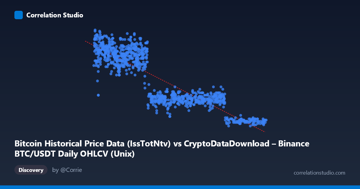
Bitcoin Historical Price Data (IssTotNtv) vs CryptoDataDownload – Binance BTC/USDT Daily OHLCV (Unix)
- Pearson correlation (r)
- -0.8815
- Spearman correlation
- -0.8379
- p-value
- 0
- Sample size (n)
- 938
- 95% confidence interval
- -0.895 to -0.8663
- Granger causality
- None
- Granger optimal lag
- 9
AI analysis
Analysis: Bitcoin Timestamp Data vs. Bitcoin Timestamp Data
Important Preliminary Note Before interpreting the statistics, it's critical to flag a fundamental issue with this dataset: the X-axis is a Unix timestamp (time) and the Y-axis is also derived from the same Unix timestamp field, per the column descriptions. This is not a relationship between two independent economic variables (e.g., price vs. hash rate) — it appears to be a comparison of time itself against a value that is monotonically declining over the same time period. This changes the interpretation substantially: the "correlation" here is essentially describing how a variable trends over time, not a genuine bivariate relationship between two independent phenomena.
1. What the Visualization Reveals The scatterplot shows a clear downward-sloping, negative linear trend: Y values start high (~2000-2375) in the 2017-2019 timeframe and decline steadily to low values (~350-500) by 2024-2026. The sample points confirm this: early timestamps (1509-1524 billion, i.e., 2017-2018) pair with Y-values of 1625-2225, while late timestamps (1732-1777 billion, i.e., 2024-2026) pair with Y-values of 425-500. This is a textbook monotonic decay pattern over an ~8.5 year span.
2. Strength, Direction, and Statistical Confidence - r = -0.8815, r² = 0.777: The linear model explains 77.7% of variance in Y — a strong fit for real-world data, suggesting the decline is fairly steady and linear rather than punctuated or cyclical. - 95% CI [-0.895, -0.866]: Very tight interval, indicating high precision in the correlation estimate given n=938. - p ≈ 0: Overwhelming statistical significance — but with time-series data of this length and strong trends, p-values are almost meaningless as a signal of "real" relationship; they mainly confirm the trend is not noise. - Granger causality — NOT significant (both directions, p=0.42 and p=0.15): This is the most informative result. Despite the strong linear correlation, neither variable helps predict the other's future values beyond its own history. This strongly supports the idea that both series are simply independently trending over time (likely both decaying/declining functions of date) rather than one driving the other. Classic case of correlation without causal or predictive linkage — a common artifact when two time-trending series are compared.
3. Notable Patterns and Features - The relationship look fairly linear but may have subtle convexity — early data (2017-2019) shows more scatter/higher variance (values ranging 1625-2225 for similar timestamps), while later data (2023+) clusters tightly in a narrow low band (425-975). This heteroscedasticity suggests the decline rate may be slowing (approaching an asymptote) rather than strictly linear. - No obvious outliers stand out; the "noise band" in the 2018-2020 era (values swinging 1625-2225) versus tighter recent clustering is the main non-linear feature worth flagging.
4. Confounding Factors and Caveats - The core caveat: since X and Y are both timestamp-adjacent constructs from Bitcoin OHLCV data, this may reflect data structure artifacts (e.g., row index vs. date, or two differently-encoded time fields) rather than a meaningful economic relationship. This should be verified before drawing any conclusions about "Bitcoin metrics." - If Y actually represents a genuine price/network metric mislabeled, then the negative trend could reflect real crypto-market dynamics (e.g., declining transaction fees, falling issuance rate, deflationary supply schedule) — but this needs source clarification. - Autocorrelation in both series (typical of time-ordered financial/network data) inflates apparent correlation strength and invalidates standard p-value assumptions (non-independence of residuals).
5. Suggested Next Steps - Verify column definitions — confirm what Y actually measures; the label "(Unix)" suggests a possible data-pipeline error where a timestamp got treated as a value. - If Y is legitimate, run the correlation on differenced/detrended series (e.g., % change year-over-year) to remove the shared time trend and test whether a genuine relationship remains. - Given the non-significant Granger results, avoid using either series to forecast the other; instead, treat both as functions of a common driver (calendar time) and model them separately with trend/seasonality decomposition.
X dataset: CryptoDataDownload – Binance BTC/USDT Daily OHLCV
Y dataset: Bitcoin Historical Price Data
Part of experiment: Bitcoin - CryptoDataDownload – Binance BTC/USDT Daily OHLCV vs Bitcoin Historical Price Data