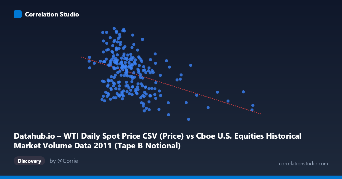
Datahub.io – WTI Daily Spot Price CSV (Price) vs Cboe U.S. Equities Historical Market Volume Data 2011 (Tape B Notional)
- Pearson correlation (r)
- -0.4013
- Spearman correlation
- -0.3527
- p-value
- 0
- Sample size (n)
- 252
- 95% confidence interval
- -0.5001 to -0.2923
- Granger causality
- None
- Granger optimal lag
- 1
AI analysis
Scatterplot Analysis: WTI Crude Oil Price vs. Cboe Tape B Notional Volume (2011)
Relationship Overview The scatterplot reveals a modest negative relationship between U.S. equities market notional trading volume (Tape B, X-axis) and WTI crude oil spot prices (Y-axis) across 252 trading days in 2011. As equity market volume increases, oil prices tend to drift lower, though the scatter is substantial and the linear fit (y = -1.805×10⁻⁹x + 104.11) captures only a fraction of the data's variability. The relationship is visually noisy, with considerable vertical spread at most volume levels, suggesting that other forces are driving oil prices independently of equity market activity.
Correlation Strength and Statistical Significance The Pearson correlation of r = -0.4013 indicates a weak-to-moderate inverse association, but the variance explained statistic tells a more sobering story: R² = 0.161, meaning equity trading volume accounts for only about 16% of the variance in WTI prices. The remaining 84% is attributable to factors entirely outside this model. The 95% confidence interval of [-0.50, -0.29] confirms the negative direction is reliable and does not cross zero, and the p-value of 3.6×10⁻¹¹ is highly significant given a population of N = 3,780 — statistical significance here is partly a function of the large sample base rather than effect size alone. Critically, the Granger causality tests show no significant predictive directionality in either direction (X→Y: p = 0.81; Y→X: p = 0.13), meaning that neither variable meaningfully predicts the other's future values at a one-period lag. The correlation, while real, appears to be contemporaneous and potentially spurious rather than causally structured.
Notable Patterns and Outliers Several features stand out in the data. The bulk of observations cluster in the X range of roughly 3–6 billion in notional volume, with oil prices spanning a wide band between ~85 and ~112 USD/barrel within that zone — illustrating the weak predictive power visually. A handful of high-volume outliers (notably near 9.5–10 billion and one approaching 14 billion) anchor the right tail and pull the regression slope downward; these extreme volume days correspond to lower oil prices, consistent with risk-off equity market conditions. There is also a visible lower-left void — days with both low volume and low oil prices are absent — and a cluster of relatively high oil prices (105–113) concentrated at lower volume levels (~3–4.5 billion), which drives much of the negative slope. The distribution does not appear strongly non-linear, but the heteroscedasticity in the middle volume range warrants attention.
Confounding Factors and Caveats This correlation almost certainly reflects shared macroeconomic drivers rather than a direct mechanism between equity volume and oil prices. In 2011, markets were shaped by the Eurozone debt crisis, Arab Spring supply disruptions, U.S. debt ceiling debates, and Federal Reserve policy — all of which could simultaneously suppress equity volumes during risk-on periods (when oil was also bid up) and spike volumes during sell-offs (when oil fell). The Tape B designation (NYSE American and regional exchanges) adds another layer: Tape B volume is a subset of total market activity and may reflect different dynamics than broad market volume. Additionally, the use of daily data without lag adjustment means any cross-market feedback operating on intraday or multi-day timescales would be invisible here, and the absence of Granger causality cautions strongly against any directional interpretation.
Actionable Insights and Further Investigation Given that only 16% of variance is explained and no causal direction is established, this correlation should not be used as a standalone trading signal. However, several follow-up analyses are warranted: (1) Include broader market volume (Tape A + C) and VIX as covariates to test whether the correlation survives controls for market-wide risk sentiment; (2) Segment by event regimes (e.g., Eurozone crisis episodes vs. calm periods) to test whether the correlation is driven by specific macro stress windows; (3) Explore lagged correlations at 2–10 periods to check whether the Granger null holds across longer lags; and (4) Test non-linear or threshold models, as the relationship may strengthen only during high-volatility regimes. The 2011 single-year window also limits generalizability — replicating across multiple years would clarify whether this is a structural relationship or a year-specific artifact.
X dataset: Cboe U.S. Equities Historical Market Volume Data 2011
Y dataset: Datahub.io – WTI Daily Spot Price CSV
Part of experiment: Daily - Cboe U.S. Equities Historical Market Volume Data 2011 vs Datahub.io – WTI Daily Spot Price CSV