World Bank CO2 Emissions by Country (DataBank) (Liquid Fuel) vs Population, Total for United States (POPTOTUSA647NWDB) (POPTOTUSA647NWDB)
- Pearson correlation (r)
- 0.732
- Spearman correlation
- 0.7649
- p-value
- 0
- Sample size (n)
- 61
- 95% confidence interval
- 0.5886 to 0.8307
- Granger causality
- None
- Granger optimal lag
- 10
AI analysis
Scatterplot Analysis: U.S. Population vs. CO₂ Emissions (Liquid Fuel)
Relationship Overview
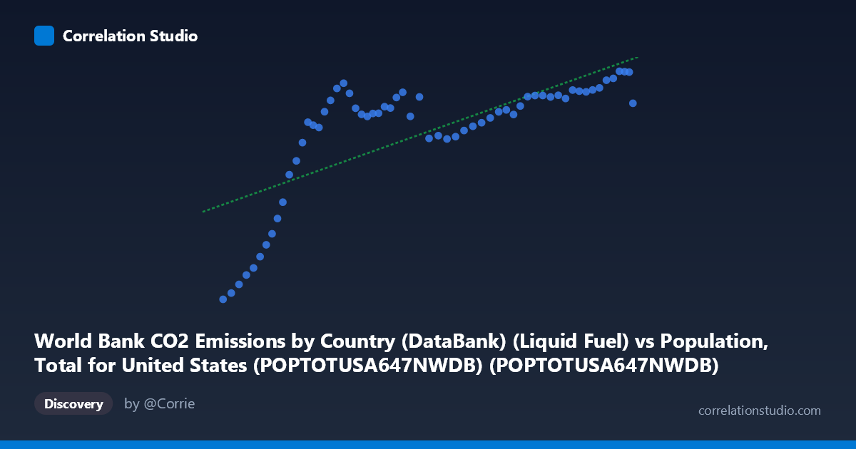
The scatterplot reveals a positive association between total U.S. population (X-axis) and CO₂ emissions from liquid fuel (Y-axis) over the period 1960–2020. As population grows from roughly 181 million to 332 million, liquid fuel CO₂ emissions generally rise from approximately 4,448 to a peak near 13,600 units. The linear regression equation (y = 3.88×10⁻⁵x + 1,240.21) suggests that each additional million people in the U.S. corresponds to roughly 38.8 units of additional liquid fuel CO₂ emissions, though the relationship is clearly not purely linear across all population ranges.
Correlation Strength and Statistical Significance
The Pearson correlation of r = 0.732 indicates a moderately strong positive relationship, but the coefficient of determination r² = 0.5358 tells a more sobering story: population size explains only about 53.6% of the variance in liquid fuel CO₂ emissions, meaning nearly half the variation is attributable to other factors entirely. The 95% confidence interval for r spans [0.589, 0.831], confirming that the true correlation is meaningfully positive but with non-trivial uncertainty. The p-value of 2.05×10⁻¹¹ makes it statistically clear this association is not due to chance. However, the Granger causality results are notably weak — neither X→Y (F=1.54, p=0.175) nor Y→X (F=0.92, p=0.530) achieves significance even at a 10-period lag. This means population growth does not temporally predict subsequent changes in emissions in a statistically defensible way, and vice versa, urging caution against any causal narrative.
Notable Patterns, Clusters, and Outliers
The scatterplot exhibits a visually distinct two-regime structure. At lower population values (roughly 180–210 million, corresponding to the early 1960s), emissions are disproportionately low (4,448–10,000 range), creating a steep, almost hockey-stick rise. Once the population exceeds approximately 220–230 million, the relationship flattens considerably into a dense cluster where emissions hover between ~11,000 and ~13,600 regardless of further population growth. Several early-period points — particularly those near (180,671,000; 4,447), (183,691,000; 4,700), and (186,538,000; 5,047) — appear as low-emission outliers relative to the regression line, pulling the fit and inflating the apparent correlation. Conversely, the upper-right cluster of high-population, high-emission points (300 million population) shows tight grouping, suggesting near-saturation of emissions growth in recent decades.
Confounding Factors and Interpretation Caveats
The correlation almost certainly reflects shared temporal trends rather than a direct mechanistic link between headcount and liquid fuel emissions. Both variables trend upward over time as part of long-run economic development, meaning time itself (or GDP, industrialization, and energy infrastructure) is a powerful lurking variable. The dramatic saturation observed after ~230 million population likely corresponds to real-world shifts: fuel efficiency standards (CAFE regulations post-1975 oil crisis), structural economic changes away from manufacturing, and growing renewable energy penetration — none of which are captured by population alone. Additionally, the dataset conflates all liquid fuel CO₂ (gasoline, diesel, jet fuel, heating oil), each with distinct demand drivers. The axes are also technically swapped from the dataset labels, warranting verification that variables are correctly assigned. Finally, with 65-year time-series data, autocorrelation inflates the effective sample size and may make the p-value appear more significant than it truly is.
Actionable Insights and Further Investigation
Given that population explains barely half the emissions variance and shows no Granger-causal signal, per-capita emissions analysis would be far more revealing — isolating whether efficiency gains are genuinely decoupling emissions from population growth. Researchers should consider multivariate models incorporating GDP per capita, vehicle miles traveled, energy prices, and fuel efficiency standards as covariates. A piecewise or segmented regression would better capture the structural break visible around the 220–230 million population threshold. Testing the relationship against specific liquid fuel subcategories (e.g., gasoline vs. aviation fuel) could isolate where population pressure matters most. Finally, applying first-differencing or detrending before correlation analysis would remove the shared temporal trend and yield a more honest estimate of whether population changes genuinely co-move with emissions changes year-over-year.
X dataset: Population, Total for United States (POPTOTUSA647NWDB)
Y dataset: World Bank CO2 Emissions by Country (DataBank)
Part of experiment: Yearly - Population, Total for United States (POPTOTUSA647NWDB) vs World Bank CO2 Emissions by Country (DataBank)