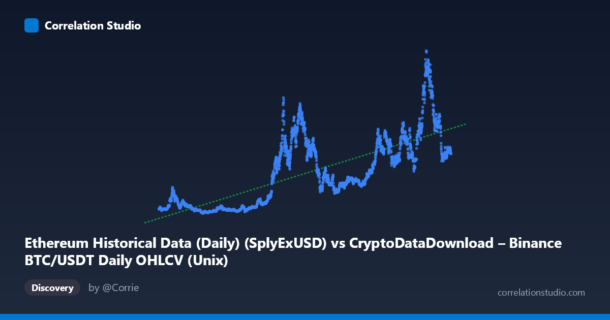
Ethereum Historical Data (Daily) (SplyExUSD) vs CryptoDataDownload – Binance BTC/USDT Daily OHLCV (Unix)
- Pearson correlation (r)
- 0.7519
- Spearman correlation
- 0.7824
- p-value
- 0
- Sample size (n)
- 3191
- 95% confidence interval
- 0.7364 to 0.7666
- Granger causality
- None
- Granger optimal lag
- 10
AI analysis
Analysis: Time vs. Ethereum Metric Relationship
Important caveat first: Despite the column labels referencing "SplyExUSD" and "Unix" timestamps for BTC/USDT OHLCV data, the actual X-axis values (ranging from ~1.5 trillion to ~1.78 trillion) are clearly Unix millisecond timestamps spanning August 2017 to May 2026. This means the visualization is effectively plotting a metric against time itself, not two independent market variables. This mislabeling significantly affects how the statistics should be interpreted.
1. What the Visualization Reveals
With X being a time index, this scatterplot is essentially a time series trend chart. The Y variable (ranging from ~1.4B to ~95.6B) shows a general upward trajectory over the 2017–2026 period, but with substantial cyclicality rather than steady growth. Sample points show low values (~2.4–5.4B) clustered in 2019–2020 and 2023, contrasted with high values (~40–95B) in late 2021, 2022, and 2025–2026 — consistent with known crypto market boom-bust cycles.
2. Strength and Direction of Correlation
The correlation (r = 0.752, r² = 0.565) indicates a moderate-to-strong positive linear trend over time, with the linear model explaining 56.5% of variance. The tight confidence interval [0.736, 0.766] and p-value effectively at 0 confirm this trend is statistically robust, not a sampling artifact — unsurprising given n=3,191. However, since X is time, this r² essentially quantifies long-term growth/drift, not a causal or predictive relationship between two independent phenomena. The remaining ~43.5% of variance reflects the strong cyclical/volatile behavior that a simple linear fit cannot capture (evident in the wide swings between consecutive sample points, e.g., 2022's ~34B dropping to 2023's ~3.6–5B, then surging past 80B by 2025).
The Granger causality results (p=0.118 and p=0.337, both non-significant) are not meaningfully interpretable here since Granger tests assume two distinct time series with a shared time axis — with X itself being time, this test is somewhat degenerate. Treat this result as uninformative rather than evidence of "no relationship."
3. Notable Patterns and Non-Linear Features
The data clearly exhibits multiple boom-bust cycles rather than monotonic growth: - A trough around 2019–2020 (values near 2–6B) - A sharp rise into 2021–2022 (peaking ~30–42B) - A pullback in 2023 (back to ~4–20B range) - Renewed acceleration into 2024–2026, with the highest sampled values (75–95B) appearing near 2025–2026
This is classic cyclical/exponential-with-corrections behavior typical of crypto asset valuations, gas fees, or network activity metrics — not a linear process. A linear fit will systematically underpredict during peaks and overpredict during troughs.
4. Confounding Factors and Caveats
- Metadata mismatch: The axis descriptions don't match the actual data (timestamps vs. described OHLCV/supply metrics), so any causal or economic interpretation should be treated cautiously until the true variable identities are confirmed. - Autocorrelation: With X being time, r² is inflated by trend/drift; both series (X trivially, Y substantially) are non-stationary, which can produce spurious high correlation even absent genuine structural relationship. - Cyclicality: Bull/bear market regimes (2018, 2021, 2022, 2024–25) act as a lurking factor driving Y, unrelated to elapsed time per se — it's driven by market sentiment, halving cycles, macro liquidity, etc.
5. Suggested Next Steps
1. Verify column mapping — confirm whether X truly represents a timestamp or was mislabeled during export; if it's genuinely a market variable, redo the analysis with correct data. 2. Detrend and test stationarity (ADF/KPSS) before drawing correlation conclusions; consider using year-over-year differences or log returns instead of raw levels. 3. Segment by market cycle/halving epoch to see if the relationship is stable or regime-dependent. 4. Use non-linear or piecewise models (e.g., polynomial, spline, or regime-switching) to better capture the cyclical growth pattern rather than a single linear fit.
X dataset: CryptoDataDownload – Binance BTC/USDT Daily OHLCV
Y dataset: Ethereum Historical Data (Daily)
Part of experiment: Bitcoin - CryptoDataDownload – Binance BTC/USDT Daily OHLCV vs Ethereum Historical Data (Daily)