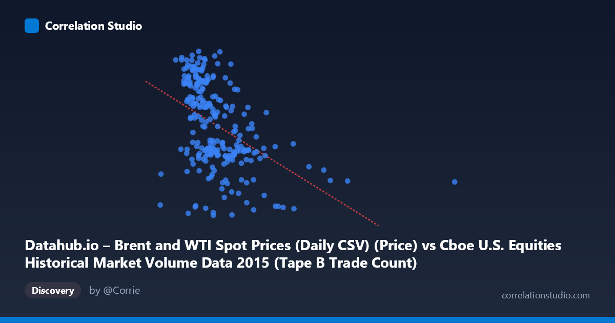
Datahub.io – Brent and WTI Spot Prices (Daily CSV) (Price) vs Cboe U.S. Equities Historical Market Volume Data 2015 (Tape B Trade Count)
- Pearson correlation (r)
- -0.4573
- Spearman correlation
- -0.516
- p-value
- 0
- Sample size (n)
- 251
- 95% confidence interval
- -0.55 to -0.3535
- Granger causality
- None
- Granger optimal lag
- 1
AI analysis
Analysis: Brent Crude Oil Prices vs. Cboe Tape B Trade Count (2015)
Relationship Overview The scatterplot reveals a moderate negative relationship between U.S. equity market trading volume (Tape B trade count, on the X-axis) and Brent crude oil spot prices (Y-axis) across 251 trading days in 2015. As trading volume increases, oil prices tend to decline. The linear regression equation (y = −3.907×10⁻⁵x + 63.998) suggests that for every one million additional trades, Brent crude prices fall by approximately $39 per barrel in a purely linear sense — though this mechanical interpretation should be treated cautiously given the nature of these variables. The overall visual impression is of a downward-sloping cloud with considerable scatter, consistent with a real but far from deterministic relationship.
Correlation Strength, Direction, and Causality The Pearson correlation of r = −0.457 indicates a moderate negative association, statistically highly significant (p = 2.24×10⁻¹⁴). However, the coefficient of determination R² = 0.209 reveals that only ~21% of the variance in Brent crude prices is explained by Tape B trade count, leaving roughly 79% of price variation attributable to other factors. The 95% confidence interval [−0.550, −0.354] is meaningfully below zero across its entire range, confirming the negative direction is robust and not a sampling artifact. Critically, Granger causality tests find no significant predictive directionality in either direction (X→Y: F = 1.27, p = 0.260; Y→X: F = 1.35, p = 0.247), meaning that past values of trading volume do not help forecast oil prices, and vice versa. This strongly suggests the correlation reflects a shared response to common drivers rather than any direct causal link between these variables.
Patterns, Clusters, and Outliers Several structural features are visible in the data. The bulk of observations cluster in the 130,000–450,000 trade count range, where the negative trend is most apparent and oil prices span roughly 35–67 USD/barrel. A handful of high-volume outliers extend well beyond 500,000 trades (reaching ~1,014,000), consistently associated with lower oil prices in the 40–49 USD range, pulling the regression line and amplifying the apparent correlation. These extreme-volume days likely correspond to market stress events — high-volatility sessions in 2015 when equity markets surged in activity (e.g., August 2015 correction). Within the main cluster, the relationship is noisier and less defined, with substantial vertical spread at any given volume level, suggesting the correlation is heavily influenced by these tail observations.
Confounding Factors and Caveats The most important caveat is that 2015 was a structurally unusual year for both variables simultaneously: Brent crude prices fell dramatically from ~65 USD in January to ~36 USD by year-end due to OPEC supply decisions and a global glut, while U.S. equity markets experienced elevated volatility and elevated volume spikes, particularly in Q3. This creates a spurious temporal confound — both series trend in their respective directions across the calendar year, and any two trending variables measured over the same period will appear correlated. Additionally, the dataset description labels are swapped in presentation (X-axis described as oil price data but labeled as market volume, and vice versa), warranting careful verification of variable assignment before drawing conclusions. The N = 3,302 population size versus n = 251 sample also raises questions about the sampling methodology.
Actionable Insights and Further Investigation Given the lack of Granger causality, practitioners should resist using equity trading volume as a leading indicator for oil prices (or the reverse) in short-term forecasting models. Further investigation should include: (1) controlling for calendar time to isolate whether the correlation persists after detrending both series, which would test whether the relationship is genuine or purely a 2015 temporal artifact; (2) segmenting the analysis by quarter to determine whether the correlation is driven primarily by the high-volume outlier days in Q3; (3) including macro controls such as USD index, VIX, or equity returns to identify potential common drivers; and (4) verifying axis variable assignments to ensure data integrity. If the correlation survives detrending, exploring whether market stress indices (like VIX) serve as a latent common cause would be a productive next step.
X dataset: Cboe U.S. Equities Historical Market Volume Data 2015
Y dataset: Datahub.io – Brent and WTI Spot Prices (Daily CSV)
Part of experiment: Daily - Cboe U.S. Equities Historical Market Volume Data 2015 vs Datahub.io – Brent and WTI Spot Prices (Daily CSV)