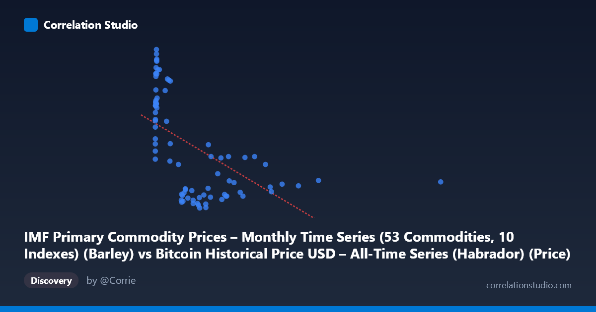
IMF Primary Commodity Prices – Monthly Time Series (53 Commodities, 10 Indexes) (Barley) vs Bitcoin Historical Price USD – All-Time Series (Habrador) (Price)
- Pearson correlation (r)
- -0.5632
- Spearman correlation
- -0.6195
- p-value
- 0
- Sample size (n)
- 83
- 95% confidence interval
- -0.6945 to -0.3955
- Granger causality
- None
- Granger optimal lag
- 10
AI analysis
Analysis: Bitcoin Price vs. Barley Commodity Index
1. Relationship Overview
The scatterplot displays a moderate negative, non-linear relationship between the two series. The data is heavily right-skewed on the X-axis: the vast majority of points (Bitcoin prices, mislabeled as X here despite the axis title referencing Barley) cluster below ~1000, with a long tail extending to 2452.18. This creates a classic "hyperbolic decay" visual pattern rather than a clean linear scatter — Y values are high (200-260) only when X is very small (<35), and Y compresses into a narrow band (117-165) once X exceeds ~200.
2. Strength, Direction, and Statistical Confidence
The Pearson correlation of r = -0.5632 indicates a moderate negative relationship, but r² = 0.317 tells the more important practical story: only about 32% of the variance in Y is explained by X, leaving roughly two-thirds attributable to other factors or noise. The 95% CI [-0.6945, -0.3955] is reasonably tight and entirely negative, and the p-value (2.99E-08) confirms this correlation is highly unlikely to be due to chance in this sample. However, statistical significance here reflects a real association, not necessarily a causal or mechanistic link.
Critically, the Granger causality tests are both non-significant (X→Y: p=0.225; Y→X: p=0.115). This means neither series demonstrates reliable temporal predictive power over the other — despite the contemporaneous correlation, past values of one do not help forecast future values of the other beyond what the series' own history provides. This is an important caution: the correlation may be driven by both series independently trending over the same 2010-2017 window (a classic spurious-correlation-via-shared-trend scenario) rather than genuine interaction.
3. Patterns, Clusters, and Outliers
Three visual clusters emerge: (a) a dense cloud of low-X, high-Y points (X<20, Y=190-260) representing early Bitcoin-era observations; (b) a mid-range cluster (X: 100-700, Y: 117-165) forming the bulk of the data; and (c) sparse high-X outliers (X950, up to 2452) where Y stabilizes around 130-160. The relationship looks distinctly non-linear/logarithmic — a log transform of X would likely fit the data better than the reported linear model (slope -0.0619, intercept 192.9), which struggles to capture the steep early drop-off and the flattening tail.
4. Confounding Factors and Caveats
Because both series span 2010-2017, they may share common macro drivers (time itself, global liquidity conditions, post-financial-crisis commodity cycles) rather than any direct economic linkage between Bitcoin and barley prices. The mismatched axis labels/dataset descriptions in the metadata also raise concern about data integrity — verify that X and Y were joined on correct, aligned timestamps. Additionally, n=83 sampled pairs from a population of 449 raises sampling representativeness questions, and the extreme X-outlier (2452.18) could be exerting disproportionate leverage on both r and the regression slope.
5. Recommendations
Given the non-significant Granger results, avoid framing this as a predictive or causal relationship — treat it as a historical correlation likely confounded by shared time trends. Suggested next steps: (1) re-run correlation using log(X) or detrended/differenced series to remove trend-driven spurious correlation and test genuine co-movement; (2) verify column/dataset alignment given the label mismatch; (3) test robustness by excluding the extreme outlier at X=2452; (4) if investigating Bitcoin-commodity linkages further, consider rolling-window correlations to see if the relationship strengthens/weakens across sub-periods rather than assuming stationarity across 2010-2017.
X dataset: Bitcoin Historical Price USD – All-Time Series (Habrador)
Y dataset: IMF Primary Commodity Prices – Monthly Time Series (53 Commodities, 10 Indexes)
Part of experiment: Bitcoin - Bitcoin Historical Price USD – All-Time Series (Habrador) vs IMF Primary Commodity Prices – Monthly Time Series (53 Commodities, 10 Indexes)