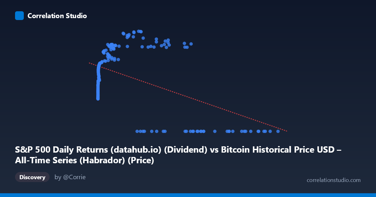
S&P 500 Daily Returns (datahub.io) (Dividend) vs Bitcoin Historical Price USD – All-Time Series (Habrador) (Price)
- Pearson correlation (r)
- -0.5041
- Spearman correlation
- 0.036
- p-value
- 0
- Sample size (n)
- 189
- 95% confidence interval
- -0.6034 to -0.3894
- Granger causality
- X → Y
- Granger optimal lag
- 4
AI analysis
Analysis of Bitcoin Price vs. S&P 500 Return Metric Relationship
1. Overview of the Relationship
The scatterplot reveals a distinctly non-linear pattern that a simple correlation coefficient struggles to capture. At low X values (roughly 0–1,500), Y rises steeply and appears logarithmically related to X, climbing from ~22 to ~46 as X increases across just a few orders of magnitude. However, once X exceeds ~30,000–40,000, the data bifurcates sharply: one cluster continues the upward trend (Y in the 55–69 range), while a large secondary cluster collapses to Y=0 regardless of X value, even at very high X (up to 118,670). This bimodal split at high X values is the dominant visual feature of the chart and is not well-described by a single linear model.
2. Correlation Strength and Statistical Interpretation
The Pearson correlation of r = -0.504 indicates a moderate negative linear relationship, with r² = 0.254 meaning only about 25% of the variance in Y is explained by a linear function of X — the majority (75%) is driven by other factors or non-linear dynamics. The 95% CI [-0.603, -0.389] is reasonably tight and excludes zero, and the p-value (1.4×10⁻¹³) confirms this relationship is highly unlikely to be due to chance. However, the negative linear slope is somewhat misleading given the visual pattern: it's largely an artifact of the Y=0 cluster at high X values dragging the linear fit downward, rather than a genuine monotonic decline. The Granger causality result (X→Y significant at p=0.029, lag=4; Y→X not significant at p=0.116) suggests X has some temporal predictive power over Y, but the modest F-statistic (2.76) indicates this predictive relationship is weak-to-moderate rather than strong.
3. Notable Patterns and Outliers
The most striking feature is the "floor" of Y=0 values appearing across a wide swath of high X values (27,983 to 118,670) — this is not noise but a structural regime, possibly representing a specific market condition, missing data encoded as zero, or a distinct period (e.g., dividend suspension, delisting, or a data artifact) coexisting with periods where X reaches similar magnitudes but Y remains high (57–69). This suggests X alone doesn't determine Y — there's likely a time-dependent or regime-dependent third factor separating these two behaviors at the same X level. The low-X region, by contrast, shows a clean, smooth, monotonically increasing (likely logarithmic) relationship with no zero values.
4. Caveats and Confounders
The variable naming is confusing/mismatched (X-axis labeled as "S&P 500 Daily Returns" pulling from the Bitcoin dataset, Y-axis labeled as Bitcoin price pulling from S&P dataset) — this metadata inconsistency raises concern about whether columns were correctly joined/aligned. Given the 16-year time coverage (2010–2026) and highly skewed X distribution (mean 20,533 vs. median likely much lower, stdev 29,894), this is almost certainly Bitcoin price data merged with an S&P-derived series by date, and the "zero" cluster may reflect a specific historical period (e.g., pre-2013 when one series had no data or was literally zero/null). Linear regression is a poor fit here given the clear non-linearity and bimodal split; r² should be interpreted cautiously as it underrepresents the true structure.
5. Recommendations
Before drawing conclusions, verify the data pipeline/column mapping given the swapped-looking labels. Segment the analysis by the apparent regime split (Y=0 vs. Y0 cluster) and investigate whether this corresponds to a specific date range — a time-series plot (not just scatter) would clarify whether the Y=0 values cluster in a particular period. Consider log-transforming X given its wide range and right skew, and fit a non-linear (logarithmic or piecewise) model instead of linear regression to better capture the true relationship. Finally, since Granger causality suggests weak X→Y predictability at a 4-period lag, this warrants deeper time-series analysis (e.g., VAR modeling) rather than relying on static correlation alone.
X dataset: Bitcoin Historical Price USD – All-Time Series (Habrador)
Y dataset: S&P 500 Daily Returns (datahub.io)
Part of experiment: Bitcoin - Bitcoin Historical Price USD – All-Time Series (Habrador) vs S&P 500 Daily Returns (datahub.io)