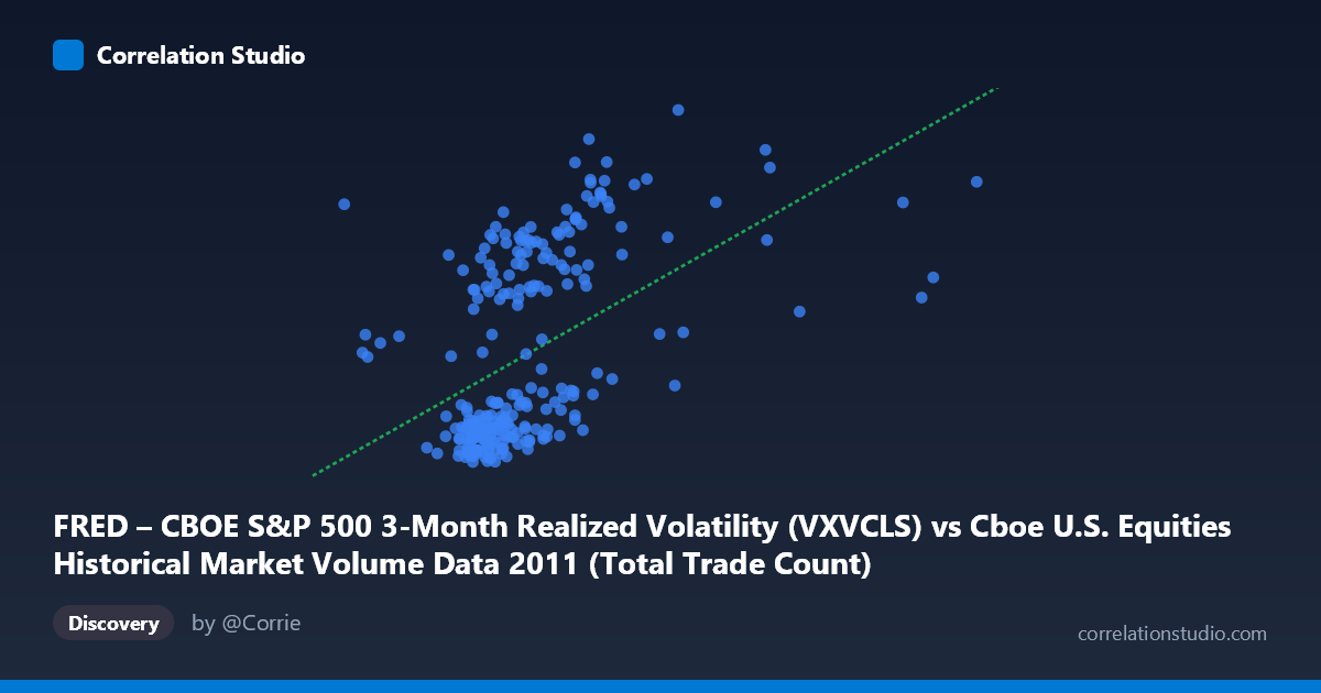
FRED – CBOE S&P 500 3-Month Realized Volatility (VXVCLS) vs Cboe U.S. Equities Historical Market Volume Data 2011 (Total Trade Count)
- Pearson correlation (r)
- 0.4922
- Spearman correlation
- 0.5897
- p-value
- 0
- Sample size (n)
- 252
- 95% confidence interval
- 0.3925 to 0.5805
- Granger causality
- None
- Granger optimal lag
- 1
AI analysis
Analysis: CBOE S&P 500 3-Month Realized Volatility vs. Total Trade Count (2011)
Relationship Overview The scatterplot reveals a positive relationship between CBOE S&P 500 3-Month Realized Volatility (VXVCLS) and Total Trade Count in U.S. equities markets during 2011. As volatility increases, trade counts tend to rise as well — a directionally intuitive finding, since periods of market turbulence typically drive heightened trading activity. The linear regression equation (y = 6.37×10⁻⁶x + 12.48) confirms this upward slope, though the relationship is clearly imperfect, with substantial scatter visible throughout the plot. The data spans a full calendar year (January 3 to December 30, 2011), capturing meaningful market episodes including the European sovereign debt crisis and the U.S. debt ceiling debate, which likely contributed volatility spikes observed in the sample points (e.g., trade counts reaching 41.24 and 38.18 at high X values).
Correlation Strength and Statistical Significance The Pearson correlation of r = 0.4922 indicates a moderate positive association, but the explanatory power is importantly limited: r² = 0.2423 means only ~24.2% of the variance in volatility (Y) is explained by trade count (X). The remaining ~75.8% of variation is attributable to other factors entirely. The 95% confidence interval of [0.3925, 0.5805] is reasonably tight given n = 252, confirming that the true population correlation is unlikely to be trivially small or near-perfect — it is genuinely moderate. The p-value of effectively zero confirms the correlation is statistically significant and not a sampling artifact. However, Granger causality analysis tells a critical story: neither direction of temporal prediction is significant (X→Y: F = 0.0008, p = 0.977; Y→X: F = 0.1655, p = 0.685). This means trade volume does not predict future volatility, and volatility does not predict future trade counts in any temporally leading sense at the 1-period lag tested — the relationship is contemporaneous rather than predictive.
Patterns, Clusters, and Outliers The scatterplot exhibits a notable bimodal or clustered structure. A dense concentration of points appears at lower X values (roughly 1,500,000–2,200,000 trade counts) with Y volatility values in the 17.5–25 range, suggesting a baseline "calm market" regime that dominated much of 2011. A second, more dispersed cluster emerges at higher Y values (30–43), corresponding to elevated volatility episodes, where X values span a wider range. Several prominent outliers are visible in the sample: the point at (2,438,164, 41.24) represents an extreme volatility reading with only moderate trade volume, while (2,540,145, 38.18) and (2,517,220, 37.04) form a high-volatility cluster. The relationship also appears to have non-linear characteristics — the variance in Y expands considerably at higher X values (heteroscedasticity), suggesting a simple linear model may underfit the true dynamics, particularly during stress periods.
Confounding Factors and Caveats Several important caveats temper interpretation. First, axis labeling appears to have the datasets swapped — the X-axis is labeled as VXVCLS (volatility) but the dataset description references market volume, and vice versa for Y — which warrants verification before drawing firm conclusions. Second, causality cannot be established from this correlation; both variables likely respond simultaneously to common market-wide shocks (e.g., macro news events, Fed announcements), making confounding by a third variable the most plausible explanation for their co-movement. Third, temporal autocorrelation within daily financial time series means the effective degrees of freedom are lower than n = 252 implies, potentially overstating statistical precision. Fourth, the N = 3,780 population figure suggests this sample is drawn from a larger dataset, and sampling methodology could introduce selection effects. Finally, regime changes within 2011 (pre- vs. post-August debt ceiling crisis) likely produce structurally different relationships that a single linear model obscures.
Actionable Insights and Further Investigation Practitioners and researchers should pursue several follow-up analyses. Regime-based segmentation — splitting the data into low- and high-volatility periods (e.g., VIX above/below 25) — would likely reveal stronger within-regime correlations and clarify whether the relationship is driven primarily by crisis episodes. Non-linear modeling (e.g., polynomial regression, spline fits, or GARCH-type models) should be tested given the apparent heteroscedasticity. Since Granger causality at lag-1 is insignificant, testing longer lags (2–5 periods) or intraday data could uncover lead-lag dynamics not visible at daily frequency. Additionally, controlling for confounders such as VIX levels, macro announcement days, and options expiration dates would help isolate the genuine volume-volatility nexus. Finally, verifying the axis dataset assignments is an immediate priority to ensure the directional interpretation is physically meaningful.
X dataset: Cboe U.S. Equities Historical Market Volume Data 2011
Y dataset: FRED – CBOE S&P 500 3-Month Realized Volatility
Part of experiment: Daily - Cboe U.S. Equities Historical Market Volume Data 2011 vs FRED – CBOE S&P 500 3-Month Realized Volatility