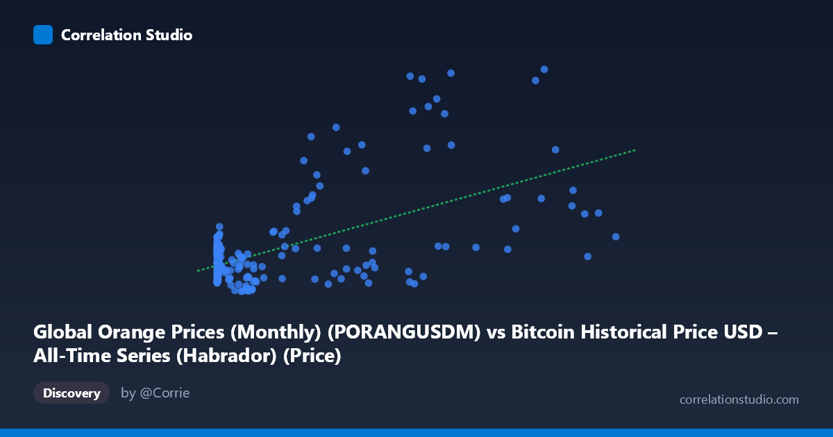
Global Orange Prices (Monthly) (PORANGUSDM) vs Bitcoin Historical Price USD – All-Time Series (Habrador) (Price)
- Pearson correlation (r)
- 0.5765
- Spearman correlation
- 0.331
- p-value
- 0
- Sample size (n)
- 189
- 95% confidence interval
- 0.4727 to 0.6646
- Granger causality
- None
- Granger optimal lag
- 1
AI analysis
Analysis: Bitcoin Price vs. Global Orange Prices
1. Relationship Overview
The scatterplot shows a positive but noisy association between Bitcoin price (X-axis, spanning a massive range from $0.06 to $118,670) and global orange prices (Y-axis, $0.97–$5.10/metric ton index). The data reveals a highly skewed X distribution—the vast majority of points cluster below $10,000, with a long tail extending to Bitcoin's all-time highs. Y values increase modestly as X increases, but with substantial scatter at every X level, particularly in the mid-to-high Bitcoin price range ($20,000–$100,000+), where orange prices vary widely from ~1.1 to 5.1.
2. Strength, Direction, and Statistical Uncertainty
The correlation coefficient (r = 0.58) indicates a moderate positive linear relationship, but r² = 0.337 means only 33.7% of the variance in orange prices is explained by Bitcoin price—leaving nearly two-thirds unexplained by this simple linear model. The 95% CI [0.477, 0.668] is reasonably tight given the sample size (n=188) and excludes zero, and the p-value ≈ 0 confirms this correlation is statistically significant and not due to chance. However, statistical significance ≠ practical strength or causation. Critically, the Granger causality tests show no significant predictive direction either way (X→Y: p=0.47; Y→X: p=0.46). This strongly suggests the correlation is not driven by one variable temporally leading the other—more likely both are responding to a shared underlying trend (e.g., time itself, global monetary conditions, or inflation) rather than one causing the other.
3. Notable Patterns and Outliers
Several features stand out: - Heteroscedasticity: Variance in Y increases substantially as X grows. At low Bitcoin prices (<$1,000), orange prices stay tightly clustered near 1.2–1.8. At high Bitcoin prices ($50,000), Y ranges enormously (1.1 to 5.1). - High-Y outliers at high-X: Points like (97365, 5.10), (57454, 4.97), (60981, 4.92) show orange prices spiking when Bitcoin is elevated—but counterexamples like (58724.66, 1.11) and (45092.81, 1.12) show high Bitcoin with low orange prices, undermining a clean linear story. - Dense low-X cluster: Most sub-$1,000 Bitcoin observations correspond to Bitcoin's early years (2010s), when orange prices were also in a narrower historical band. - The relationship looks more like two variables trending upward together over time rather than a direct functional dependency—consistent with the Granger results.
4. Confounding Factors and Caveats
This pairing is a classic case of spurious correlation via a shared time trend. Bitcoin's price grew exponentially from 2010–2026, and global commodity prices (including oranges) have also risen due to unrelated factors: inflation, agricultural supply shocks (citrus greening disease, weather events in Brazil/Florida), currency effects (USD strength), and general commodity price cycles. Both series are non-stationary time series with strong upward drift, which commonly inflates correlation coefficients without implying any causal or economic linkage. The linear regression (y = 1.75e-5·x + 1.45) is also questionable given the extreme skew in X (mean $20,280 vs. median likely far lower)—log-transforming X would likely be more appropriate and could substantially change the apparent relationship.
5. Recommendations for Further Investigation
- Detrend or difference both series (e.g., use returns/percentage changes instead of levels) and re-run correlation and Granger tests to check if the relationship survives—this is the standard fix for spurious time-trend correlation. - Log-transform Bitcoin price given its multi-order-of-magnitude range, and re-fit the regression. - Introduce a common time-trend control variable or use cointegration testing to properly assess whether these series share a long-run equilibrium relationship versus merely coincidental drift. - Treat this correlation as not actionable for trading or forecasting purposes—the lack of Granger causality in either direction confirms Bitcoin price should not be used to predict orange prices or vice versa.
X dataset: Bitcoin Historical Price USD – All-Time Series (Habrador)
Y dataset: Global Orange Prices (Monthly)
Part of experiment: Bitcoin - Bitcoin Historical Price USD – All-Time Series (Habrador) vs Global Orange Prices (Monthly)