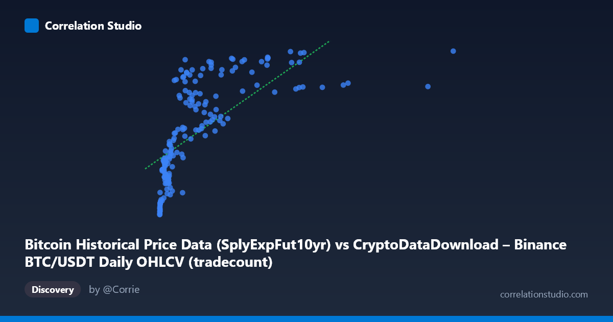
Bitcoin Historical Price Data (SplyExpFut10yr) vs CryptoDataDownload – Binance BTC/USDT Daily OHLCV (tradecount)
- Pearson correlation (r)
- 0.6799
- Spearman correlation
- 0.8822
- p-value
- 0
- Sample size (n)
- 180
- 95% confidence interval
- 0.5926 to 0.7514
- Granger causality
- None
- Granger optimal lag
- 10
AI analysis
Analysis of Bitcoin Price/Supply Metric vs. Trade Count Relationship
1. Overall Relationship
The scatterplot reveals a positive but distinctly non-linear relationship between the X variable (SplyExpFut10yr, a Bitcoin supply-related metric ranging from near-zero to ~10.1M) and Y (tradecount, ranging from ~20.2M to ~20.8M). The data shows a classic saturating/logarithmic curve shape: Y rises steeply as X increases from near-zero to roughly 2-3 million, then flattens dramatically, with Y values clustering tightly between 20.5M-20.8M even as X extends out to 10 million. This "diminishing returns" pattern is visually the dominant feature of the plot.
2. Strength, Direction, and Statistical Confidence
The Pearson correlation (r = 0.68) indicates a moderately strong positive linear association, with r² = 0.46 meaning the linear model explains only 46% of the variance in Y — leaving over half unexplained by a straight-line fit. The 95% CI [0.59, 0.75] is reasonably tight and excludes zero, and the p-value ≈ 0 confirms this correlation is highly unlikely to be due to chance given n=180. However, the note that Spearman ρ exceeds Pearson r is a critical flag: it confirms the visual impression that a monotonic non-linear relationship (log or power curve) fits the data better than the linear model, meaning the true explanatory power of X on Y is likely higher than 46% once curvature is properly modeled. Critically, the Granger causality tests (p = 0.30 and p = 0.47, both non-significant) show that neither variable temporally predicts the other in this panel — meaning despite the contemporaneous correlation, X's past values do not help forecast future Y values, and vice versa. This suggests the relationship, whatever its shape, is not a simple lead-lag dynamic.
3. Notable Patterns and Outliers
The most striking pattern is the steep early rise: points with X < 500,000 span a wide range of Y (20.2M-20.7M), showing high sensitivity in this low-X region. Beyond X ≈ 3,000,000, Y essentially plateaus near 20.75M-20.8M regardless of further X increases (e.g., X=10,085,578 yields Y=20,828,425 — barely higher than X=1,770,765 at Y=20,786,275). There's also a secondary cluster of low-Y, low-X points (X<20,000, Y≈20.2M-20.3M) representing an early/baseline regime, and a couple of mid-range X points with comparatively lower Y (e.g., X=785,996, Y=20,292,625) that deviate from the general upward trend, suggesting some volatility or regime-dependent behavior in the low-to-mid X range.
4. Confounding Factors and Caveats
Both series are likely driven by a common underlying trend — time/Bitcoin network maturation — since X is a supply-expansion metric and Y is trade count, both of which naturally grow (or saturate) as the Bitcoin market matures. This makes the correlation potentially spurious or mediated by an omitted "market growth/adoption" variable rather than reflecting genuine causal linkage. The tradecount metric may also be influenced by exchange-specific factors (Binance volume, API changes, bot activity) unrelated to the supply metric. Additionally, the non-stationarity implied by both series trending over the 2017-2026 window can inflate correlation estimates and undermine the Granger test's reliability if differencing wasn't applied.
5. Recommendations for Further Investigation
Given the log-like saturation pattern, refit using a logarithmic or power transformation on X (e.g., regress Y on ln(X)) to better capture the true r² and relationship shape. Test both series for stationarity (ADF test) and consider differencing before rerunning Granger causality, since trending data can mask or distort lag-based causal signals. Segment the analysis by X regime (e.g., X < 1M vs. X 3M) to explore whether the relationship's strength/shape differs meaningfully across phases of Bitcoin's supply expansion, and investigate whether a third variable (e.g., overall market cap or active addresses) better explains the shared variance in both series.
X dataset: CryptoDataDownload – Binance BTC/USDT Daily OHLCV
Y dataset: Bitcoin Historical Price Data
Part of experiment: Bitcoin - CryptoDataDownload – Binance BTC/USDT Daily OHLCV vs Bitcoin Historical Price Data