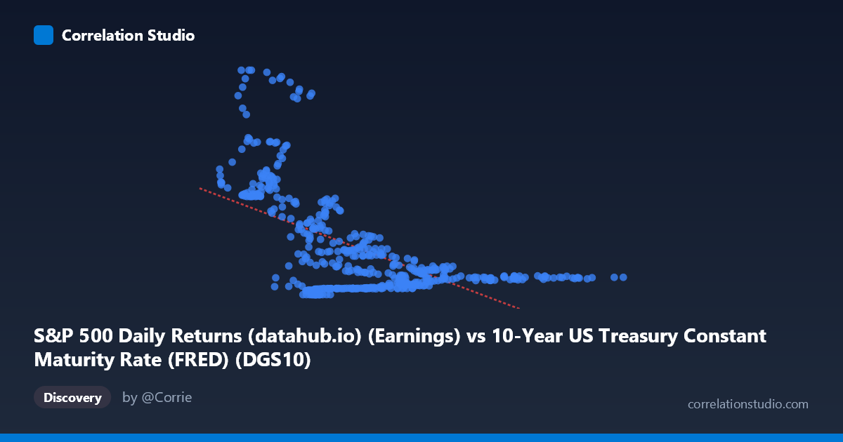
S&P 500 Daily Returns (datahub.io) (Earnings) vs 10-Year US Treasury Constant Maturity Rate (FRED) (DGS10)
- Pearson correlation (r)
- -0.5816
- Spearman correlation
- -0.4718
- p-value
- 0
- Sample size (n)
- 493
- 95% confidence interval
- -0.6371 to -0.5199
- Granger causality
- None
- Granger optimal lag
- 1
AI analysis
Analysis: S&P 500 Earnings vs. 10-Year Treasury Yield (1962–2026)
1. Overall Relationship The scatterplot reveals a moderate negative relationship between the 10-Year US Treasury Constant Maturity Rate (X-axis) and S&P 500 Earnings (Y-axis), captured by the regression equation y = -8.87x + 92.60. This means that as Treasury yields rise, S&P 500 earnings tend to be lower in this paired dataset — though the relationship is far from deterministic. The plot shows substantial vertical scatter at every X value, indicating that Treasury yields alone leave much of the earnings variation unexplained. Notably, the highest earnings values (approaching ~190-197) cluster at very low yield levels (below ~3), while moderate-to-high yield ranges show compressed, lower earnings values.
2. Correlation Strength and Statistical Significance The correlation of r = -0.582 reflects a moderate negative association, but the more telling metric is r² = 0.338, meaning Treasury yields statistically explain only about 33.8% of the variance in S&P 500 earnings — leaving roughly two-thirds of variation attributable to other factors. The 95% confidence interval of [-0.637, -0.520] is relatively tight and entirely negative, lending strong confidence that the negative direction is genuine rather than a sampling artifact. The p-value of effectively zero (across N = 1,865 observations) confirms the relationship is highly statistically significant. However, the Granger causality results are notably null in both directions (X→Y: F ≈ 0.00, p = 0.996; Y→X: F = 1.00, p = 0.318), meaning neither variable meaningfully predicts the future values of the other at a 1-period lag. This is a critical distinction: the cross-sectional correlation is real, but there is no evidence of a temporal predictive relationship, undermining any causal narrative.
3. Patterns, Clusters, and Outliers Several structural features stand out in the point cloud. There is a clear high-scatter cluster at low X values (0.6–3.0), where earnings range wildly from near zero to ~197 — suggesting that low-yield environments coincide with highly variable earnings conditions, likely spanning different economic eras (e.g., early 1960s low-rate periods vs. post-2008 zero-rate environments). By contrast, the mid-to-high yield range (7–15) shows a much tighter, compressed cluster of earnings values predominantly between 0 and ~25, consistent with the high-rate era of the late 1970s–1980s when earnings were relatively modest in real terms. Several notable outliers exist at low X values — points like (2.39, 196.03), (3.26, 187.23), and (1.48, 182.91) — which likely represent recent post-pandemic earnings spikes in a suppressed-rate environment and exert considerable leverage on the regression line.
4. Confounding Factors and Caveats This relationship is heavily confounded by time and historical regime effects. The data spans over 60 years (1962–2026), during which both earnings and interest rates underwent dramatic structural shifts driven by inflation cycles, Federal Reserve policy regimes, tax law changes, and corporate profit margin expansion. The apparent negative correlation may largely reflect two distinct eras superimposed: a high-rate / low-earnings era (1970s–1980s) and a low-rate / high-earnings era (2010s–2020s), rather than a direct mechanical relationship. This makes the correlation potentially spurious or confounded by shared secular trends. Additionally, the axis labels appear inverted from what one might expect (earnings on Y, yields on X), and the dataset note suggests the columns may have been swapped during merging — worth verifying. The non-linear dispersion at low X values also suggests a linear model is likely misspecified for this data.
5. Actionable Insights and Further Investigation Given the absence of Granger causality, practitioners should resist using Treasury yields as a near-term predictor of earnings in any trading or forecasting model. More productive next steps would include: (1) segmenting the analysis by decade or Fed policy regime to test whether the correlation holds within sub-periods or is purely a cross-era artifact; (2) testing non-linear models (e.g., piecewise regression or regime-switching models) to better capture the heteroskedastic spread visible at low yields; (3) incorporating inflation-adjusted (real) earnings and real yields to remove the shared inflation component driving both series; and (4) exploring multivariate models that add GDP growth, profit margins, or credit spreads to isolate the incremental explanatory power of yields. The strong outliers at low X should also be examined individually to determine whether they represent data quality issues or genuinely extreme economic episodes requiring separate treatment.
X dataset: 10-Year US Treasury Constant Maturity Rate (FRED)
Y dataset: S&P 500 Daily Returns (datahub.io)
Part of experiment: Daily - 10-Year US Treasury Constant Maturity Rate (FRED) vs S&P 500 Daily Returns (datahub.io)