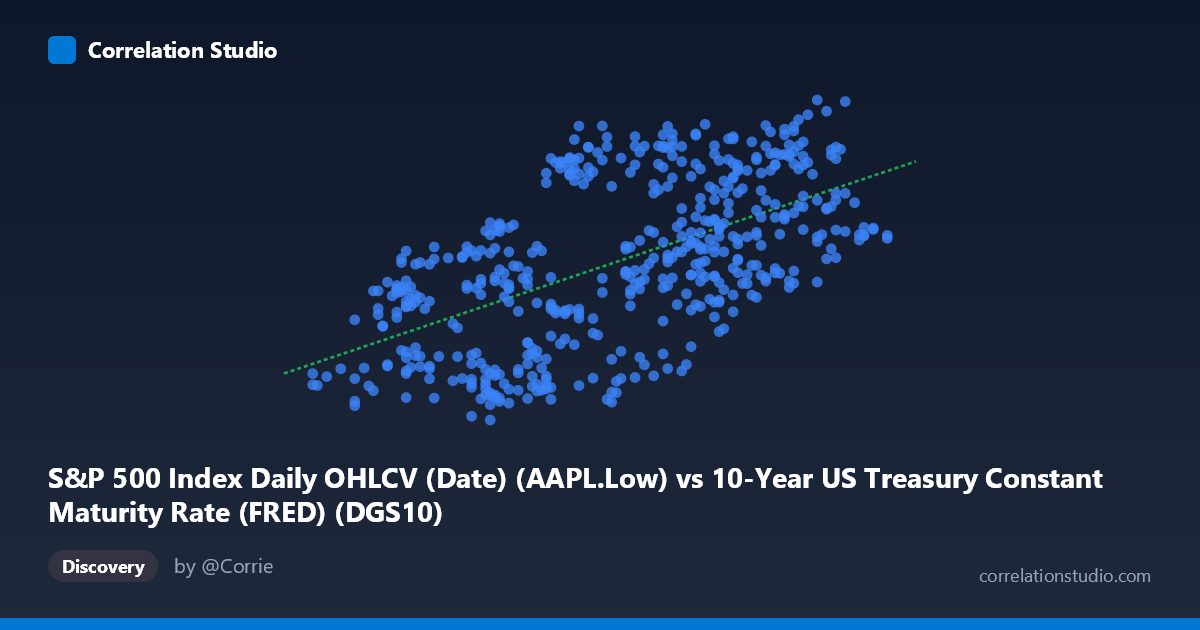
S&P 500 Index Daily OHLCV (Date) (AAPL.Low) vs 10-Year US Treasury Constant Maturity Rate (FRED) (DGS10)
- Pearson correlation (r)
- 0.5796
- Spearman correlation
- 0.592
- p-value
- 0
- Sample size (n)
- 502
- 95% confidence interval
- 0.5184 to 0.6349
- Granger causality
- X → Y
- Granger optimal lag
- 1
AI analysis
Analysis: AAPL Low Price vs. 10-Year US Treasury Yield (2015–2017)
Relationship Overview The scatterplot reveals a moderate positive relationship between Apple's daily low price (X-axis) and the 10-year US Treasury constant maturity rate (Y-axis) over the two-year period from February 2015 to February 2017. The linear regression equation (y = 22.23x + 66.98) indicates that for every $1 increase in AAPL's low price, the 10-year Treasury yield is associated with a roughly 22-basis-point increase. While this directional trend is visible in the data, the scatter around the regression line is substantial, signaling that the relationship is real but far from deterministic.
Correlation Strength and Statistical Significance The Pearson correlation of r = 0.58 represents a moderate positive association, but the more telling statistic is r² = 0.336 — meaning only 33.6% of the variance in Treasury yields is explained by AAPL's low price. The remaining ~66% is driven by other factors entirely. The 95% confidence interval of [0.518, 0.635] is reasonably tight and excludes zero, and the p-value is effectively zero (p < 0.001 across n = 502 paired observations), confirming the correlation is statistically robust and not a sampling artifact. Critically, the Granger causality test supports a unidirectional temporal relationship: X (AAPL Low) Granger-causes Y (Treasury yield) at a 1-period lag (F = 6.93, p = 0.009), while the reverse direction fails to reach significance (F = 2.85, p = 0.092). This suggests that past AAPL price movements carry incremental predictive information about future Treasury yield movements — a counterintuitive but statistically meaningful finding worth scrutinizing carefully.
Patterns, Clusters, and Outliers The sample points reveal notable clustering at two ends of the distribution. A lower cluster around AAPL Low ≈ $1.53–$1.80 shows Treasury yields spanning a wide range (~91–116), indicating high variability at lower price levels. A higher cluster around $2.20–$2.50 tends to show elevated yields (110–135), consistent with the positive slope. Several apparent outliers stand out: the point at (1.90, 125.91) and (1.56, 112.34) sit well above the regression line for their X values, while (2.01, 92.00) and (1.86, 93.69) fall considerably below it. These deviations suggest periods where macroeconomic events temporarily decoupled the two series. The spread also appears to widen at higher X values, hinting at possible heteroscedasticity that a simple linear model may not fully capture.
Confounding Factors and Caveats The most significant interpretive caveat here is the dataset label mismatch: the X-axis is labeled as AAPL Low prices sourced from a Treasury rate dataset, and the Y-axis as Treasury yields sourced from an S&P 500 dataset — suggesting a possible data alignment or labeling error that warrants verification before drawing firm conclusions. Beyond that, both variables are time-series data embedded in a shared macroeconomic environment (2015–2017), meaning any correlation may be spurious co-movement driven by common underlying forces — such as the Federal Reserve's rate normalization cycle beginning in late 2015, broad equity market conditions, or risk-on/risk-off sentiment cycles — rather than any genuine causal link. The Granger causality result, while statistically significant, does not imply economic causation; it may reflect shared sensitivity to a third variable (e.g., economic growth expectations) that manifests in equity prices slightly before bond markets reprice.
Actionable Insights and Further Investigation Given the Granger causality finding, a productive next step would be to introduce control variables — particularly the Federal Funds Rate, S&P 500 index level, and VIX — into a multivariate regression to test whether the AAPL→yield predictive relationship survives. Researchers should also apply cointegration testing (e.g., Engle-Granger or Johansen) to determine whether a long-run equilibrium relationship exists between these series, and test for structural breaks around the December 2015 Fed rate hike. A rolling-window correlation analysis would clarify whether the r = 0.58 relationship is stable across the full period or concentrated in specific sub-periods. Finally, resolving the apparent dataset labeling inconsistency is essential before any findings are used for decision-making or publication.
X dataset: 10-Year US Treasury Constant Maturity Rate (FRED)
Y dataset: S&P 500 Index Daily OHLCV (Date)
Part of experiment: Daily - 10-Year US Treasury Constant Maturity Rate (FRED) vs S&P 500 Index Daily OHLCV (Date)