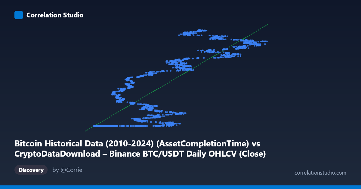
Bitcoin Historical Data (2010-2024) (AssetCompletionTime) vs CryptoDataDownload – Binance BTC/USDT Daily OHLCV (Close)

Pearson correlation (r): 0.8518
Spearman correlation: 0.8876
p-value: 0
Sample size (n): 3191
95% confidence interval: 0.842 to 0.861
Granger causality: None
Granger optimal lag: 10
Time coverage: 2017-08-17 to 2026-05-20

AI analysis

Analysis: Bitcoin "Asset Completion Time" vs. BTC/USDT Close Price

1. What the Visualization Reveals

The scatterplot shows a moderately strong positive relationship between the X-axis variable (labeled as "AssetCompletionTime," though the values—ranging from ~3,189 to ~124,658—appear to be a numeric field, possibly a transaction/completion metric rather than a timestamp) and BTC/USDT closing price. The data shows a distinctive pattern: a dense cluster of points where X is small (roughly 3,000–25,000) and Y is compressed near the minimum (~1,614,337,000), followed by a more dispersed, upward-trending scatter as X increases beyond ~25,000. This suggests a floor effect or regime change rather than a uniform linear relationship across the full range.

2. Strength, Direction, and Statistical Meaning

The correlation coefficient (r = 0.852) indicates a strong positive linear association, with r² = 0.726 meaning 72.6% of the variance in Y is explained by X — a substantial but not complete explanatory relationship, leaving ~27% of variance driven by other factors. The 95% CI [0.842, 0.861] is tight, and the p-value of ~0 confirms this correlation is highly statistically significant and not due to chance, especially given the large sample size (n=3,191).

However, the Granger causality tests are critical here: neither direction shows significant predictive causality (X→Y: p=0.326; Y→X: p=0.168). This means despite the strong contemporaneous correlation, X does not temporally predict future Y, nor vice versa. This is an important distinction — the relationship is associative/concurrent, not predictive or causal in a time-series sense. Practically, this correlation should not be used for forecasting one variable from lagged values of the other.

3. Notable Patterns and Non-linearities

The chart reveals at least two distinct behaviors: - A flat/compressed cluster at low X values (~3,000–25,000) where Y sits tightly near 1,614,337,000–1,614,338,000, suggesting many data points correspond to a fixed or early-period price floor. - A fanning, positively-sloped scatter for X 25,000, where Y climbs toward 1,780,000,000 with increasing variance — indicating heteroscedasticity (variance in Y grows as X increases).

This pattern resembles a threshold or piecewise relationship rather than a single clean linear trend, which the linear R² may be partially capturing due to the separation between the low-X cluster and the high-X spread rather than a true continuous linear process.

4. Confounding Factors and Caveats

- Time confound: Since this spans 2017–2026, both variables likely trend with overall Bitcoin market cycles (bull/bear markets), making the correlation potentially spurious or mediated by time/market regime rather than a direct causal link. - Variable definition ambiguity: The X-axis label ("AssetCompletionTime") and its numeric range don't clearly align with a standard "completion time" metric — clarification of what this field represents is needed before drawing domain conclusions. - Non-stationarity: Bitcoin prices are notoriously non-stationary; both series may share unit-root behavior, which can inflate correlation and r² without implying genuine relationship (classic spurious regression risk in time series). - Clustering artifact: The dense flat cluster at low X may disproportionately anchor the regression and inflate apparent fit.

5. Actionable Insights and Next Steps

- Clarify the X-variable definition — confirm whether "AssetCompletionTime" is a timestamp, duration, or index, as this fundamentally changes interpretation. - Test for stationarity (ADF/KPSS tests) on both series before trusting correlation/Granger results, and consider differencing or detrending to check if the relationship holds beyond shared trend. - Segment the analysis by regime (the low-X flat cluster vs. high-X fanning region) — a piecewise or non-linear model (e.g., spline, log transform) may fit better than a single linear regression. - Given the lack of Granger causality, avoid using this relationship for predictive/trading signals; treat it as descriptive/correlational only. - Investigate a third common driver (e.g., calendar time, market volume, or macro BTC price cycle) that may explain both variables simultaneously.

X dataset: CryptoDataDownload – Binance BTC/USDT Daily OHLCV

Y dataset: Bitcoin Historical Data (2010-2024)

Part of experiment: Bitcoin - CryptoDataDownload – Binance BTC/USDT Daily OHLCV vs Bitcoin Historical Data (2010-2024)