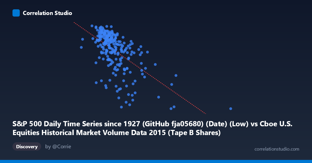
S&P 500 Daily Time Series since 1927 (GitHub fja05680) (Date) (Low) vs Cboe U.S. Equities Historical Market Volume Data 2015 (Tape B Shares)
- Pearson correlation (r)
- -0.5988
- Spearman correlation
- -0.5918
- p-value
- 0
- Sample size (n)
- 252
- 95% confidence interval
- -0.6726 to -0.5132
- Granger causality
- X → Y
- Granger optimal lag
- 7
AI analysis
Scatterplot Analysis: S&P 500 Daily Low vs. Cboe Tape B Share Volume (2015)
Relationship Overview
The scatterplot reveals a moderate negative relationship between the S&P 500 daily low price (X-axis) and Cboe Tape B share volume (Y-axis) across 252 trading days in 2015. As the S&P 500's daily low price increases, Tape B share volume tends to decrease, tracing a downward-sloping linear trend captured by the regression equation y = -1.2133×10⁻⁶x + 2174.82. The visual pattern shows a reasonably coherent negative slope, though with substantial scatter around the regression line, indicating the relationship is real but far from deterministic. The X variable spans a wide range (~44M to ~312M, though concentrated between ~65M–135M), while Y clusters predominantly between ~1,900 and ~2,130 shares, suggesting most observations fall within a dense central band with meaningful dispersion on both axes.
Correlation Strength, Direction, and Statistical Significance
With r = -0.5988, the correlation is moderate-to-strong in direction — negative — and statistically robust. The r² = 0.3586 indicates that approximately 35.9% of the variance in Tape B share volume is explained by the S&P 500 daily low, leaving roughly 64% attributable to other factors. While not trivial, this means the majority of volume variation remains unexplained by price level alone. The 95% confidence interval of [-0.6726, -0.5132] is meaningfully narrow given the sample size of 252, confirming the negative correlation is not a statistical artifact — the true population correlation almost certainly lies in negative territory. The p-value of ~0 (against N = 3,302 and n = 252) makes this association highly significant. Critically, Granger causality runs unidirectionally from X→Y (F = 2.1848, p = 0.0364) at an optimal lag of 7 trading periods (~1.5 weeks), meaning S&P 500 daily lows have statistically significant temporal predictive power over future Tape B volume, while the reverse (Y→X: F = 0.5531, p = 0.7934) shows no predictive relationship. This asymmetry is practically meaningful: lower index price levels appear to precede elevated trading volumes in subsequent days, consistent with market stress dynamics.
Notable Patterns, Clusters, and Outliers
Several features stand out in the scatter distribution. The bulk of observations cluster between X = 70M–130M and Y = 1,950–2,130, forming a relatively dense core. A few notable outliers are visible at extreme X or Y values: the point near (205M–213M, ~1,867–1,971) at the far right represents unusually high S&P 500 daily lows paired with low Tape B volumes, consistent with late-2015 elevated price levels when volatility was lower. Conversely, points with Y below ~1,900 (e.g., ~1,867 and ~1,879) at X values around 130M–205M may reflect specific low-volume episodes possibly tied to holiday-shortened sessions or post-volatility exhaustion. The spread noticeably widens at lower X values, hinting at possible heteroscedasticity — when the S&P 500 was trading at lower levels (consistent with August 2015 volatility), Tape B volumes were both higher and more variable, suggesting non-constant variance along the regression line. There is no strong evidence of a non-linear relationship from the sample points, but the funnel-shaped dispersion warrants attention.
Confounding Factors and Interpretive Caveats
Several important caveats complicate causal interpretation. 2015 was not a uniform market year — it included the August 2015 "flash crash" and significant late-summer volatility, which simultaneously depressed S&P 500 price levels and dramatically spiked trading volumes. This means the correlation may be largely driven by a single volatility episode rather than a stable structural relationship, making it period-specific. Additionally, Tape B shares represent a specific subset of U.S. equity volume (NYSE American/AMEX-listed securities), which may have its own compositional dynamics not representative of total market activity. The Granger causality result, while statistically significant, uses an F-statistic only marginally above the threshold (p = 0.0364), suggesting the predictive edge is real but not overwhelming — and Granger causality does not imply true economic causation. Finally, both variables are jointly driven by broader macro and sentiment factors (VIX, Federal Reserve communications, global risk-off events), making it difficult to isolate a direct price-to-volume mechanism.
Actionable Insights and Further Investigation
The 7-period Granger lag is particularly actionable: traders or risk managers could investigate whether S&P 500 daily lows below certain thresholds (e.g., below ~1,950) serve as leading indicators for Tape B volume spikes 7 days forward, potentially useful for liquidity forecasting or execution timing in AMEX-listed securities. To deepen this analysis, it would be worthwhile to: (1) segment the data by volatility regime (pre- vs. post-August 2015 flash crash) to test whether the correlation is structurally stable or event-driven; (2) control for VIX as a confounder to isolate price-level effects from fear/uncertainty effects on volume; (3) test nonlinear models (e.g., piecewise regression or GAM) to capture potential threshold effects visible in the heteroscedastic scatter; and (4) replicate across multiple years to determine whether the negative price-volume relationship in Tape B is persistent or a 2015-specific artifact driven by the unique volatility environment of that year.
X dataset: Cboe U.S. Equities Historical Market Volume Data 2015
Y dataset: S&P 500 Daily Time Series since 1927 (GitHub fja05680) (Date)
Part of experiment: Daily - Cboe U.S. Equities Historical Market Volume Data 2015 vs S&P 500 Daily Time Series since 1927 (GitHub fja05680) (Date)