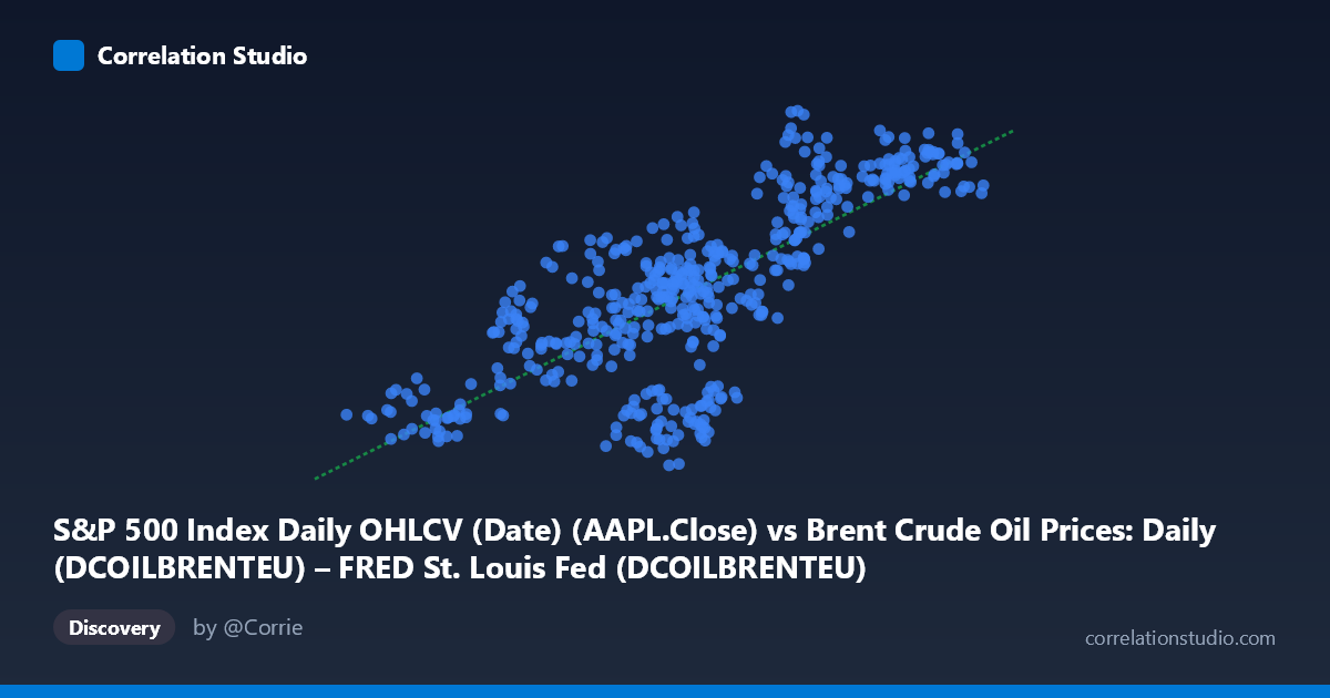
S&P 500 Index Daily OHLCV (Date) (AAPL.Close) vs Brent Crude Oil Prices: Daily (DCOILBRENTEU) – FRED St. Louis Fed (DCOILBRENTEU)

Pearson correlation (r): 0.7646
Spearman correlation: 0.7607
p-value: 0
Sample size (n): 504
95% confidence interval: 0.7257 to 0.7986
Granger causality: None
Granger optimal lag: 1

AI analysis

Scatterplot Analysis: AAPL Close Price vs. Brent Crude Oil Price (2015–2017)

Relationship Overview The scatterplot reveals a moderately strong positive relationship between Apple's closing stock price (X-axis) and Brent Crude Oil spot prices (Y-axis) over the two-year window from February 2015 to February 2017. As AAPL's closing price rises from roughly $26 to $66, Brent Crude tends to rise from approximately $90 to $135. The linear regression equation (y = 1.003x + 64.52) is notable for its near-unity slope, suggesting that on the scale of these variables, the two assets moved in rough lockstep during this period — a somewhat counterintuitive finding given that these assets occupy entirely different economic sectors.

Correlation Strength and Statistical Significance The Pearson correlation of r = 0.765 indicates a moderately strong positive association, but the more practically meaningful figure is r² = 0.585 — meaning that roughly 58.5% of the variance in Brent Crude prices is statistically "explained" by AAPL's closing price within this sample. While that sounds substantial, it must be interpreted cautiously. The 95% confidence interval of [0.726, 0.799] is relatively tight given n = 504, and the p-value of essentially zero confirms the correlation is highly unlikely to be a chance artifact of sampling. However, Granger causality tests tell a critical story: neither direction of temporal prediction is statistically significant (X→Y: F = 0.095, p = 0.758; Y→X: F = 0.524, p = 0.470). This means that neither variable's past values meaningfully predict the other's future values — the correlation is contemporaneous, not directional, which strongly implies a spurious or third-factor-driven relationship rather than any meaningful causal link.

Patterns, Clusters, and Outliers The scatterplot shows a broadly linear cloud with considerable vertical scatter, particularly in the mid-range of X (roughly $43–$55 AAPL), where Brent prices span nearly 40 USD/barrel (~$92 to ~$135) for similar AAPL values. This wide spread at central X values undermines confidence in practical predictive use. Several notable features emerge from the sample points: there appear to be potential clusters at lower AAPL values (≈$30–$37) with correspondingly low Brent prices (~$94–$109), and at higher AAPL values (≈$57–$66) with higher Brent prices (~$125–$129). A few candidate outliers stand out — for instance, (54.16, 135.35) and (46.08, 92.51) sit well above and below the regression line respectively, suggesting periods where the two assets temporarily diverged sharply. The overall pattern is consistent with a shared macro trend rather than a structural relationship.

Confounding Factors and Caveats The most significant caveat here is the classic spurious correlation problem: both AAPL stock and Brent Crude prices were subject to broad macroeconomic forces during 2015–2017, including global risk appetite cycles, USD strength fluctuations, and synchronized global growth trends. Both assets declined in 2015–2016 and recovered into 2016–2017, meaning much of the observed correlation likely reflects shared temporal trending (non-stationarity) rather than any structural relationship. The axis labels in the provided metadata also appear swapped — the X-axis is labeled as coming from the Brent dataset but contains AAPL price values, and vice versa — which warrants data pipeline verification before drawing any conclusions. Additionally, with daily data over just two years, the sample captures a single macro regime and may not generalize.

Actionable Insights and Further Investigation Given the absence of Granger causality and the likely spurious nature of the correlation, this relationship should not be used for trading or forecasting purposes. For further investigation, analysts should: (1) detrend or difference both series to test whether correlation persists after removing shared time trends, as cointegration analysis would be more appropriate for non-stationary financial time series; (2) extend the time window to 10+ years to test whether the correlation is regime-specific; (3) introduce control variables such as USD index, VIX, or broad market indices (S&P 500) to isolate whether the apparent link vanishes once macro factors are controlled; and (4) verify the axis/dataset mapping to ensure the variable assignment is correct before further modeling. This analysis serves as a useful reminder that high correlation between financial time series is almost never sufficient evidence of a meaningful economic relationship.

X dataset: Brent Crude Oil Prices: Daily (DCOILBRENTEU) – FRED St. Louis Fed

Y dataset: S&P 500 Index Daily OHLCV (Date)

Part of experiment: Daily - Brent Crude Oil Prices: Daily (DCOILBRENTEU) – FRED St. Louis Fed vs S&P 500 Index Daily OHLCV (Date)