VIX Volatility Index Daily (FRED) (VIXCLS) vs Cboe U.S. Equities Historical Market Volume Data 2011 (Tape A Trade Count)
- Pearson correlation (r)
- 0.6187
- Spearman correlation
- 0.6639
- p-value
- 0
- Sample size (n)
- 252
- 95% confidence interval
- 0.5361 to 0.6895
- Granger causality
- None
- Granger optimal lag
- 1
AI analysis
Analysis: VIX Volatility Index vs. Cboe Tape A Trade Count (2011)
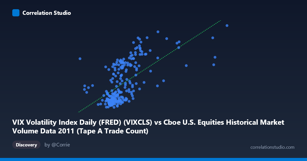
Relationship Overview The scatterplot reveals a moderate positive relationship between the VIX Volatility Index and Tape A Trade Count for U.S. equities in 2011. As the VIX rises — indicating greater implied volatility and market fear — the number of trades on Tape A tends to increase. This aligns intuitively with market microstructure theory: heightened uncertainty drives increased trading activity as investors reposition, hedge, or react to rapidly changing conditions. The linear regression equation (y = 1.594×10⁻⁵x + 5.152) suggests that for every unit increase in VIX, approximately 1.6 additional trades (scaled) are expected, though this relationship is clearly not perfectly linear.
Correlation Strength and Statistical Significance The Pearson correlation of r = 0.619 reflects a moderate positive association, but the more telling metric is r² = 0.383 — meaning VIX explains only 38.3% of the variance in Tape A Trade Count, leaving over 61% attributable to other factors. The 95% confidence interval [0.536, 0.690] is reasonably tight and does not cross zero, and the p-value of essentially 0 confirms this correlation is highly unlikely to be a chance finding in a sample of n = 252 (from a population of N = 3,780 trading days). However, Granger causality tests tell a more cautious story: neither direction (X→Y: F=0.038, p=0.845; Y→X: F=0.047, p=0.829) achieves significance at lag-1, meaning that knowing yesterday's VIX does not reliably predict today's trade count, and vice versa. This decouples statistical correlation from temporal predictive utility.
Notable Patterns, Clusters, and Outliers The scatterplot shows at least two visually distinct behavioral regimes. A dense cluster exists at lower VIX values (~14–22) where trade counts are relatively low and tightly grouped, consistent with the calm, lower-volatility periods of early-to-mid 2011. A second, more dispersed cluster emerges at higher VIX values (~28–48), corresponding to the elevated volatility during the August–October 2011 U.S. debt ceiling crisis and European sovereign debt contagion, where trade counts fan out considerably. Several potential outliers are visible at the upper right (high VIX, very high trade counts, e.g., ~2,126,541 trades at VIX ~39 and ~1,876,408 at VIX ~25), suggesting episodic volume spikes that deviate from the general trend. The relationship also appears to have a non-linear, possibly exponential character — the spread of Y values grows substantially as X increases, hinting that a log or power transformation might better capture the true functional form.
Confounding Factors and Caveats Several important caveats apply. First, 2011 was an unusually eventful year (debt ceiling debate, U.S. credit downgrade, Euro crisis), making this sample potentially non-representative of typical VIX-volume dynamics. Second, trade count on Tape A is driven by algorithmic and high-frequency trading systems that may respond to volatility in complex, nonlinear ways unrelated to investor sentiment measured by VIX. Third, day-of-week effects, options expiration cycles, and index rebalancing events could inflate both VIX and trade counts simultaneously without a direct causal link. Fourth, the Granger causality null result at lag-1 suggests both variables may be jointly driven by a common latent factor (e.g., news shocks, macroeconomic releases) rather than one causing the other. Finally, using only one year of data limits generalizability.
Actionable Insights and Further Investigation Practitioners monitoring market liquidity conditions should recognize that VIX is a useful but incomplete predictor of trading volume, capturing roughly 38% of variance — enough to be informative for risk management and execution strategy, but insufficient to rely on alone. For further investigation: (1) test higher-order lags in Granger causality (beyond lag-1) to check for delayed predictive relationships; (2) apply a log-log transformation to both variables to better model the apparent heteroscedasticity and potential power-law relationship; (3) extend the dataset across multiple years (e.g., 2008–2023) to test whether the 2011 relationship holds across different volatility regimes; and (4) incorporate additional predictors such as S&P 500 returns, bid-ask spreads, or news sentiment indices to build a more complete model of intraday trading activity dynamics.
X dataset: Cboe U.S. Equities Historical Market Volume Data 2011
Y dataset: VIX Volatility Index Daily (FRED)
Part of experiment: Daily - Cboe U.S. Equities Historical Market Volume Data 2011 vs VIX Volatility Index Daily (FRED)