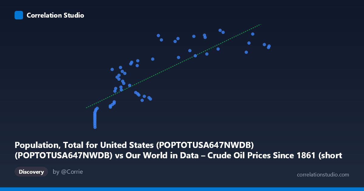
Population, Total for United States (POPTOTUSA647NWDB) (POPTOTUSA647NWDB) vs Our World in Data – Crude Oil Prices Since 1861 (short names) (oil_price_crude_current_dollars_per_m3)
- Pearson correlation (r)
- 0.8259
- Spearman correlation
- 0.8864
- p-value
- 0
- Sample size (n)
- 65
- 95% confidence interval
- 0.7288 to 0.8904
- Granger causality
- None
- Granger optimal lag
- 10
- Time coverage
- 1960-01-01 to 2024-01-01
- Recomputed on refreshed data
- 2026-10-09 (r was 0.8259)
AI analysis
Analysis: U.S. Population vs. Crude Oil Prices (1960–2024)
1. What the Visualization Reveals
The scatterplot displays a positive relationship between annual crude oil prices (X-axis, in dollars per cubic meter) and total U.S. population (Y-axis), covering 65 annual observations from 1960 to 2024. As oil prices increase, U.S. population tends to be higher, tracing a broadly upward-sloping cloud of points. However, the relationship is not cleanly linear — the distribution shows notable clustering at low oil price values and considerable scatter at moderate price ranges, suggesting that both variables are primarily being driven by their shared progression through time rather than any direct causal mechanism between them.
2. Correlation Strength, Direction, and Causal Framing
The Pearson correlation of r = 0.826 indicates a strong positive association, and the linear regression (y = 198,682x + 2.17×10⁸) reinforces this. The R² = 0.682 means that approximately 68.2% of the variance in U.S. population is statistically "explained" by oil price variation in a purely associative sense — a seemingly impressive figure that demands immediate skepticism given the subject matter. The 95% confidence interval for r of [0.729, 0.890] is relatively tight and excludes zero, and the p-value of ~0 confirms this correlation is highly unlikely to arise by chance in a sample of this size. That said, statistical significance here is almost entirely a function of both variables trending upward over six decades of shared time coverage, not any meaningful substantive link. Critically, the Granger causality tests return no significant result in either direction (X→Y: F=0.75, p=0.67; Y→X: F=1.14, p=0.37), meaning that past oil prices do not help predict future U.S. population, and vice versa. This is a decisive finding: even the modest predictive structure one might hope to extract from the correlation evaporates under temporal scrutiny.
3. Notable Patterns, Clusters, and Non-Linear Features
Several structural features stand out in the scatterplot. There is a dense cluster of points at very low oil prices (X ≈ 11–20) corresponding to lower population values in the range of roughly 180–210 million — these reflect the 1960s and early 1970s era of historically cheap oil. A second broad scatter of points spans the mid-range (X ≈ 80–350), representing the volatile oil price environment of the 1970s–2000s alongside steadily growing population. At higher oil prices (X 400), points spread more widely in the Y-direction, with population values ranging from ~295M to ~340M — capturing the 2000s and 2010s commodity boom and its aftermath. Notably, a few high-X, moderate-Y outliers (e.g., points near X ≈ 683–702 with Y ≈ 311–316M) suggest that recent high oil prices do not correspond to proportionally high population, slightly breaking the linear trend at the upper end and hinting at a plateau or ceiling effect in the relationship.
4. Confounding Factors and Interpretive Caveats
This correlation is a textbook example of a spurious time-series correlation driven by shared secular trends. Both U.S. population and nominal crude oil prices have increased substantially over the 1960–2024 period for entirely independent reasons: population grows due to births, immigration, and mortality dynamics, while oil prices respond to geopolitical events (OPEC embargoes, Gulf Wars), technological shifts (fracking, renewables), and global demand cycles. The use of nominal oil prices rather than inflation-adjusted prices further inflates the apparent correlation, since nominal values mechanically trend upward with inflation over long time horizons. The regression equation itself is nonsensical in practical terms — no analyst would credibly argue that a $1/m³ increase in oil prices causes 198,682 additional Americans to exist. The lack of Granger causality is the most honest signal in this analysis: neither series predicts the other once temporal structure is properly accounted for.
5. Actionable Insights and Further Investigation
The primary actionable insight is methodological caution: this dataset pair should not be used to support any claim about oil prices affecting population or vice versa without substantial detrending and controls. For more rigorous investigation, researchers should: (1) difference or detrend both series (e.g., use year-over-year percentage changes in oil prices and population growth rates) to remove shared trend contamination before computing correlations; (2) test whether real (inflation-adjusted) oil prices show any relationship with demographic indicators like fertility rates, migration patterns, or regional population shifts in oil-producing states; (3) explore whether oil price volatility (rather than levels) correlates with economically relevant population dynamics such as internal migration; and (4) consider multivariate models incorporating GDP, energy consumption, and policy variables to properly isolate any indirect pathways. The strong r² here should be treated as a warning sign of spurious correlation, not an invitation to causal inference.
X dataset: Our World in Data – Crude Oil Prices Since 1861 (short names)
Y dataset: Population, Total for United States (POPTOTUSA647NWDB)
Part of experiment: Yearly - Our World in Data – Crude Oil Prices Since 1861 (short names) vs Population, Total for United States (POPTOTUSA647NWDB)