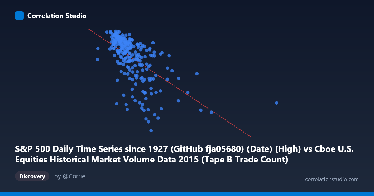
S&P 500 Daily Time Series since 1927 (GitHub fja05680) (Date) (High) vs Cboe U.S. Equities Historical Market Volume Data 2015 (Tape B Trade Count)
- Pearson correlation (r)
- -0.5886
- Spearman correlation
- -0.6574
- p-value
- 0
- Sample size (n)
- 252
- 95% confidence interval
- -0.6639 to -0.5015
- Granger causality
- None
- Granger optimal lag
- 1
AI analysis
Analysis: S&P 500 Daily High vs. Cboe Tape B Trade Count (2015)
Relationship Overview The scatterplot reveals a moderate negative relationship between the S&P 500 daily high price and the Cboe Tape B trade count across 2015 trading days. As the S&P 500 high increases, Tape B trade counts tend to decrease — suggesting that on days when equity prices were elevated, trading activity in Cboe's Tape B segment (primarily NYSE American and regional exchange-listed securities) was relatively subdued. The linear regression equation (y = −0.00032x + 2167.07) quantifies this inverse slope, with the effect being modest per unit but meaningful across the full X range spanning roughly 130,000 to over 1,000,000 in the high price series.
Correlation Strength and Statistical Interpretation The Pearson correlation of r = −0.59 indicates a moderate negative association, with r² = 0.346 meaning that approximately 34.6% of the variance in Tape B trade counts is explained by the S&P 500 daily high — leaving roughly 65% attributable to other factors. The 95% confidence interval of [−0.66, −0.50] is meaningfully narrow and entirely negative, reinforcing that the direction is consistent and not a statistical artifact. With a p-value of effectively zero across a paired sample of 252 observations drawn from a population of 3,302, this correlation is highly statistically significant. However, the Granger causality results tell a more cautious story: neither direction (X→Y nor Y→X) shows significant predictive power (F = 0.006, p = 0.94 for X→Y; F = 0.138, p = 0.71 for Y→X), meaning that past values of one variable do not help predict future values of the other. Correlation here is contemporaneous and symmetric — not directional or mechanistic in a temporal sense.
Patterns, Clusters, and Outliers The data exhibits a discernible dense cluster between roughly X = 130,000–400,000 and Y = 1,950–2,135, representing the bulk of typical trading days. Within this cluster, the negative trend is evident but noisy. Several notable outliers appear at the high end of the X-axis — points near X = 620,000–1,014,000 — which correspond to unusually high S&P 500 daily highs (or potentially data scale anomalies worth investigating). These right-tail outliers consistently show mid-range Y values rather than extreme lows, slightly moderating the regression slope. At the lower left, a few points near Y = 1,900–1,950 with moderate X values stand out as low-trade-count days, possibly associated with specific market stress events or holiday-thinned sessions in 2015 (e.g., August volatility episode).
Confounding Factors and Caveats Several important caveats apply. First, the X-axis label appears to reflect S&P 500 daily high prices, but the values range into the hundreds of thousands — this may indicate the data is in a scaled or transformed format, or there may be a unit/labeling inconsistency worth verifying before drawing firm conclusions. Second, 2015 was a specific macro environment featuring Fed rate-hike anticipation and a sharp August correction, meaning these results may not generalize to other years. Third, common temporal drivers — such as volatility regimes, end-of-quarter rebalancing, or macro announcements — could simultaneously suppress prices and inflate trade counts (or vice versa), producing a spurious correlation. Finally, Tape B specifically covers a subset of U.S. equities, so the relationship may not hold for total market volume.
Actionable Insights and Further Investigation Analysts should investigate the X-axis scale anomaly — values exceeding 500,000 for an S&P 500 "high" price are implausible at face value and may indicate a data merge error or unit mismatch. Controlling for realized volatility (VIX) as a covariate would help isolate whether the price-volume relationship persists independently of market stress. Given the absence of Granger causality, no short-term trading signal should be inferred from this correlation. A useful next step would be to segment the data by volatility regime (e.g., pre- vs. post-August 2015 correction) to test whether the negative correlation is driven by a structural break rather than a persistent relationship throughout the year.
X dataset: Cboe U.S. Equities Historical Market Volume Data 2015
Y dataset: S&P 500 Daily Time Series since 1927 (GitHub fja05680) (Date)
Part of experiment: Daily - Cboe U.S. Equities Historical Market Volume Data 2015 vs S&P 500 Daily Time Series since 1927 (GitHub fja05680) (Date)