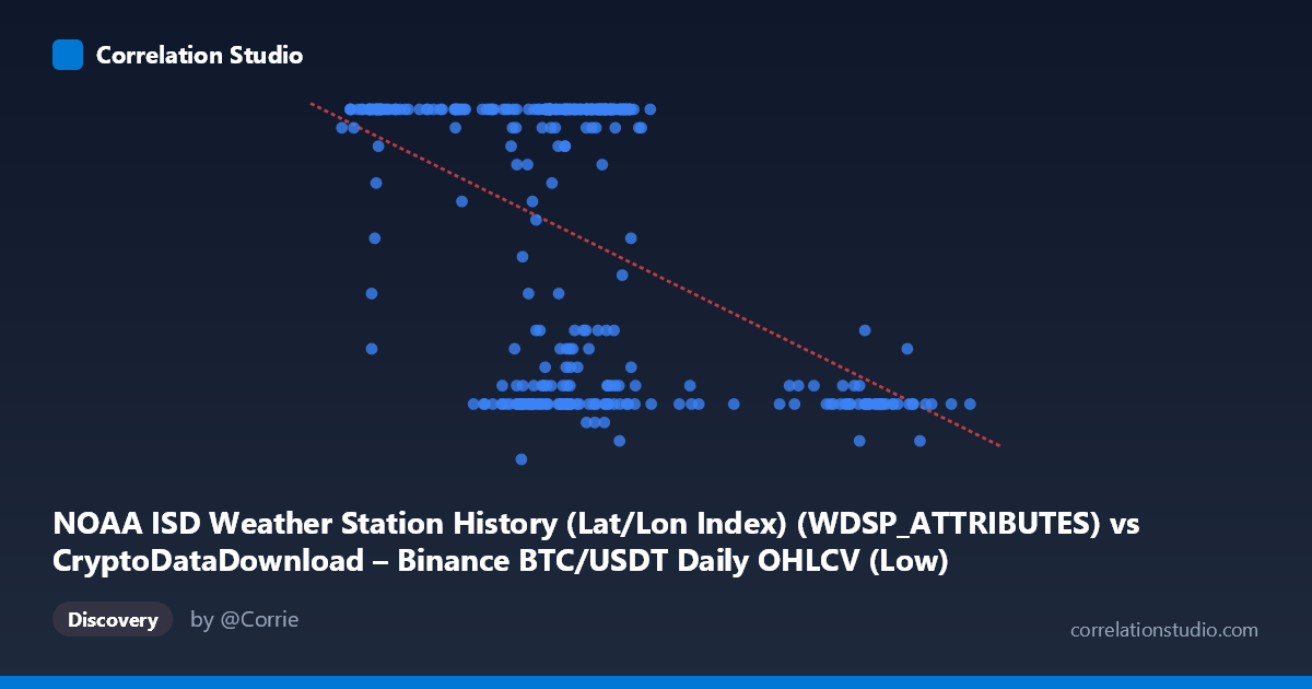
NOAA ISD Weather Station History (Lat/Lon Index) (WDSP_ATTRIBUTES) vs CryptoDataDownload – Binance BTC/USDT Daily OHLCV (Low)
- Pearson correlation (r)
- -0.4769
- Spearman correlation
- -0.3266
- p-value
- 0
- Sample size (n)
- 355
- 95% confidence interval
- -0.5535 to -0.3923
- Granger causality
- None
- Granger optimal lag
- 1
AI analysis
Analysis of the Scatterplot Relationship
1. Overview of the Visualization
The scatterplot presents a moderate negative relationship between two variables whose labeling appears to be mismatched or mislabeled in the metadata (the axis titles reference unrelated datasets — a weather station index and BTC/USDT OHLCV data — which is likely a data pipeline artifact rather than a meaningful pairing). Setting aside the label confusion, the plotted data shows X values clustered tightly between roughly 40,000–70,000, with a secondary, sparser group extending out to ~105,000. The Y variable is bounded between 5 and 24, and a large fraction of points sit at or near the ceiling value of 24, creating a dense horizontal band at the top of the chart.
2. Strength, Direction, and Statistical Confidence
The correlation coefficient (r = -0.477) indicates a moderate negative linear relationship: as X increases, Y tends to decrease. However, r² = 0.227 tells us that only about 23% of the variance in Y is explained by X — meaning roughly 77% of Y's variability is driven by other factors entirely unaccounted for in this bivariate relationship. The 95% confidence interval [-0.553, -0.392] is fairly narrow and does not cross zero, and the p-value (effectively 0) confirms this correlation is highly statistically significant and not a product of random chance, given the large sample size (n=355). That said, statistical significance should not be conflated with practical strength — this is a moderate, not strong, relationship. Critically, the Granger causality tests show no predictive direction in either direction (X→Y: p=0.657; Y→X: p=0.261), meaning that even if these were true time-series variables, neither one helps forecast future values of the other. This strongly suggests the correlation is contemporaneous/structural rather than causal or predictive.
3. Patterns, Clusters, and Outliers
The data shows clear non-random structure rather than a smooth linear cloud. Two visible clusters emerge: a dense main cluster (X: 40,000–70,000) with Y values spanning the full 5–24 range, and a sparser high-X cluster (X: 85,000–105,000) where Y values are consistently low (7–11). This creates a "stepped" or bimodal appearance rather than a continuous linear trend — the negative correlation is driven substantially by this separation between clusters rather than a uniform decline across the whole range. Additionally, many points hit the Y=24 ceiling exactly, suggesting possible data truncation, capping, or a categorical/rounded nature to Y rather than a continuous measurement. This ceiling effect at Y=24 combined with a floor cluster around Y=7-9 hints that Y may behave more like a bounded or discretized variable than a continuous one.
4. Confounding Factors and Caveats
Given the mismatched axis labels (weather station lat/lon index vs. BTC OHLCV data), it's likely these columns were incorrectly joined or represent an artifact of automated dataset pairing rather than a substantively meaningful relationship. If X is genuinely a BTC price/volume metric and Y a repeated/capped value (like a fixed attribute or day-of-month index), the "correlation" may be spurious or mechanical rather than reflecting any real-world causal mechanism. The ceiling at Y=24 and the clustering pattern both suggest structural/artificial constraints in how the data was generated or sampled, rather than organic covariation. Time coverage is a single year (2024), so no long-term trend or seasonality can be inferred, and the lack of Granger causality reinforces that this is not a temporally dynamic relationship.
5. Recommendations for Further Investigation
Before drawing substantive conclusions, verify the data provenance and confirm that X and Y are correctly mapped to their intended source columns — the label mismatch is a red flag that should be resolved first. If the variables are confirmed correct, investigate the bimodal clustering by segmenting the analysis (e.g., separate regressions for X<75,000 vs. X85,000) to determine whether the pooled correlation is being driven by a confound like time period, exchange session, or an unmeasured categorical variable. Additionally, examine why Y clusters heavily at 24 — this may indicate a capped/binned variable requiring a different modeling approach (e.g., Tobit regression or treating Y as ordinal) rather than standard OLS. Finally, given the null Granger causality result, any forecasting application should not rely on one variable to predict the other; instead, look for a third, shared driver influencing both simultaneously.
X dataset: CryptoDataDownload – Binance BTC/USDT Daily OHLCV
Y dataset: NOAA ISD Weather Station History (Lat/Lon Index)
Part of experiment: Bitcoin - CryptoDataDownload – Binance BTC/USDT Daily OHLCV vs NOAA ISD Weather Station History (Lat/Lon Index)