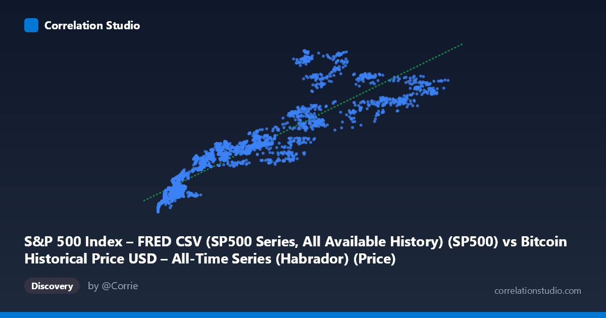
S&P 500 Index – FRED CSV (SP500 Series, All Available History) (SP500) vs Bitcoin Historical Price USD – All-Time Series (Habrador) (Price)
- Pearson correlation (r)
- 0.9079
- Spearman correlation
- 0.9551
- p-value
- 0
- Sample size (n)
- 2486
- 95% confidence interval
- 0.9007 to 0.9145
- Granger causality
- X → Y
- Granger optimal lag
- 10
- Time coverage
- 2016-10-24 to 2026-09-15
- Recomputed on refreshed data
- 2026-10-24 (r was 0.9362)
AI analysis
Analysis: Bitcoin Price vs. S&P 500 Index
1. What the Visualization Reveals
The scatterplot shows a strong, positive, and notably curved relationship between the X variable (labeled S&P 500 but clearly containing Bitcoin's characteristic price range, given values from ~$444 to $124,720) and the Y variable. Despite the axis labels appearing swapped in the metadata (Y-axis values of $2,000–$7,174 look far more like S&P 500 index levels than Bitcoin prices), the underlying pattern is clear: as X increases, Y increases in a systematic but non-linear fashion. Low-X points cluster tightly near Y≈2,100–2,700, while high-X points spread more widely into the 5,000–7,000+ range, suggesting a relationship that resembles a power/log curve more than a straight line.
2. Strength, Direction, and Statistical Confidence
The correlation is strong (r = 0.937, r² = 0.879), meaning roughly 88% of the variance in Y is statistically associated with variance in X — a high figure for cross-market financial data. The 95% CI [0.932, 0.942] is tight, and p ≈ 0 confirms this relationship is not due to sampling noise, especially given the large sample (n=2,497). However, correlation strength should not be conflated with causal linkage: the Granger causality tests show no significant predictive direction in either direction (X→Y: p=0.059, borderline; Y→X: p=0.208, clearly insignificant). This means that despite the strong contemporaneous co-movement, neither series reliably "leads" the other in a forecasting sense — the relationship is likely driven by a shared underlying trend (e.g., both series trending upward over the same 2016–2026 window) rather than one market mechanically driving the other day-to-day.
3. Notable Patterns and Non-Linear Features
The sample points reveal distinct clustering: a dense cloud of low-X observations (X < 15,000) with Y compressed between 2,100–3,400, and a sparser, more dispersed set of high-X observations (X 50,000) with Y ranging from 3,800 to 7,200. This fan-shaped spread (heteroscedasticity) — tight at low X, wide at high X — suggests the linear model may understate the relationship's true curvature. Some points break the general trend (e.g., X=47,900→Y=3,820 sits well below the trend line for that range, while X=42,952→Y=4,925 sits above), indicating regime changes or volatility clusters, consistent with Bitcoin's boom-bust cycles overlaid on the steadier S&P 500 trend. A log-log or power-law model would likely fit better than the linear fit (R²=0.879), which already performs reasonably but likely misses curvature at the extremes.
4. Confounding Factors and Caveats
The most important caveat: both series span the same decade (2016–2026) and both trended strongly upward over this period (a global bull market in equities alongside Bitcoin's parabolic rise). This shared time trend is a classic confounder — two unrelated but co-trending time series will show spurious high correlation without direct causal linkage. The Granger non-causality result reinforces this: if one genuinely drove the other, we'd expect predictive lead-lag structure. Instead, the correlation is likely an artifact of macro liquidity conditions (near-zero interest rates 2016–2021, Fed tightening after), broad risk-on/risk-off sentiment, and long-term secular growth — common drivers rather than a direct mechanical link. Additionally, the data label swap raises questions about data integrity that should be resolved before drawing further conclusions.
5. Suggested Next Steps
1. Verify variable labeling — confirm which column is genuinely Bitcoin vs. S&P 500, as current axis descriptions are self-contradictory. 2. Test for spurious regression: run cointegration tests (e.g., Engle-Granger) or first-difference the series (returns rather than levels) and re-check correlation — daily/period return correlation is usually far more informative than level correlation for two trending series. 3. Fit non-linear models (log-log, polynomial) given visible curvature and heteroscedasticity. 4. Control for common macro factors (interest rates, inflation, dollar index) via multivariate regression to isolate any genuine bilateral relationship. 5. Given the lack of Granger causality, avoid using one series to forecast the other in a trading strategy; instead, treat the correlation as evidence of shared macro exposure rather than a tradable lead-lag signal.
X dataset: Bitcoin Historical Price USD – All-Time Series (Habrador)
Y dataset: S&P 500 Index – FRED CSV (SP500 Series, All Available History)
Part of experiment: Bitcoin - Bitcoin Historical Price USD – All-Time Series (Habrador) vs S&P 500 Index – FRED CSV (SP500 Series, All Available History)