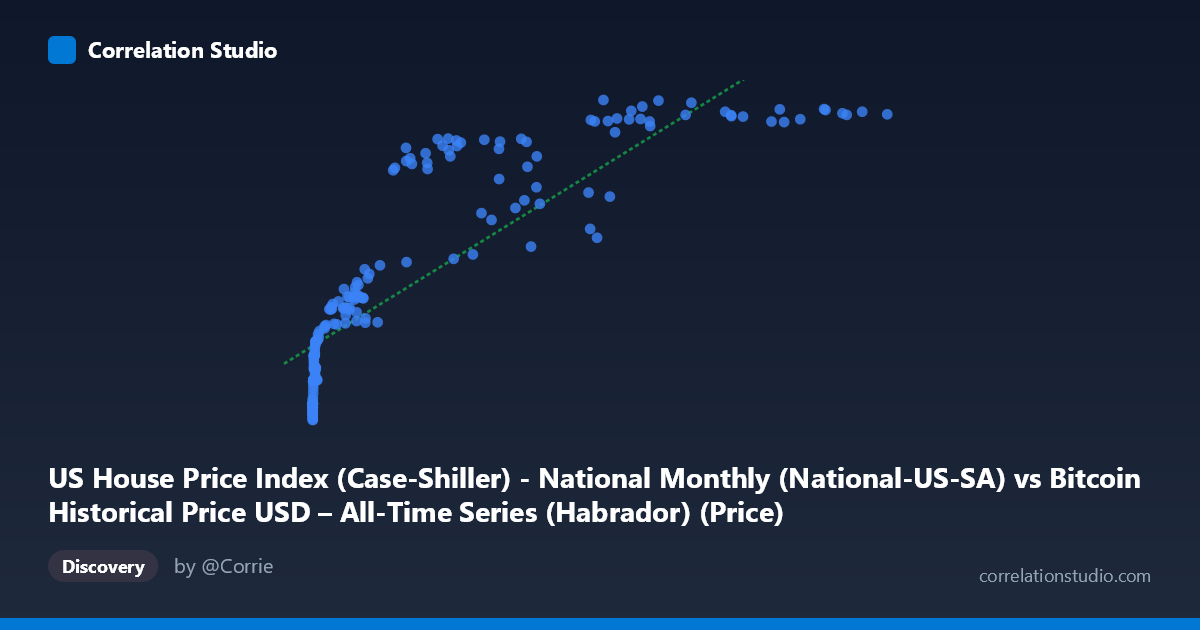
US House Price Index (Case-Shiller) - National Monthly (National-US-SA) vs Bitcoin Historical Price USD – All-Time Series (Habrador) (Price)
- Pearson correlation (r)
- 0.8503
- Spearman correlation
- 0.9707
- p-value
- 0
- Sample size (n)
- 189
- 95% confidence interval
- 0.8053 to 0.8856
- Granger causality
- None
- Granger optimal lag
- 9
AI analysis
Analysis: Bitcoin Price vs. US House Price Index (Case-Shiller National)
1. What the Visualization Reveals
The scatterplot shows a strong positive association between Bitcoin's USD price and the Case-Shiller US National Home Price Index. However, the relationship is clearly non-linear — data points trace a curve resembling a logarithmic or square-root function rather than a straight line. At low Bitcoin prices (roughly $0–$1,000), the HPI compresses into a narrow band (~135–190), while as Bitcoin climbs past $20,000–$100,000+, HPI values rise more slowly and plateau in the 290–330 range. This produces a classic "diminishing returns" curve shape rather than a proportional linear climb.
2. Strength, Direction, and Statistical Confidence
The Pearson correlation (r = 0.846, r² = 0.716) indicates a strong positive linear relationship on its face, with ~72% of the variance in one variable statistically explainable by the other. The 95% CI [0.80, 0.88] is tight and the p-value is effectively zero, meaning this correlation is highly unlikely to be due to sampling noise given the 187 paired observations. However, since Spearman's rank correlation exceeds Pearson's r, the true strength of monotonic association is understated by the linear r² — a log-transformed or polynomial fit would likely explain meaningfully more variance than the reported 71.6%.
Critically, the Granger causality tests show no significant predictive direction in either direction (X→Y: p=0.251; Y→X: p=0.102). This means neither series reliably "leads" the other in a time-lagged sense at lag 1. This is an important caveat: despite the strong contemporaneous correlation, there is no statistical evidence that house prices predict Bitcoin prices or vice versa. The relationship is likely driven by both variables trending upward over the same macro time period (2010–2026) rather than one causing the other.
3. Notable Patterns and Outliers
Several structural features stand out: - Compression at low X values: Thousands of early Bitcoin prices (near $0–$100) map to a tight HPI cluster (135–160), consistent with Bitcoin's exponential growth trajectory compressing early history into a small x-range visually. - Plateau at high X values: Once Bitcoin exceeds ~$60,000, HPI values saturate near 320–331, suggesting the housing index growth rate slowed (or reached data ceiling) while Bitcoin continued to swing wildly. - Vertical scatter at similar X: Points like (56973, 278.51) vs. (58254, 323.73) — similar Bitcoin prices but notably different HPI values — reveal that Bitcoin's boom-bust cycles (2021 crash, 2018 crash) don't align cleanly with the steadily-climbing HPI, producing "smearing" at high X.
4. Confounding Factors and Caveats
This is a textbook case of spurious correlation via shared time trend. Both series are non-stationary and generally trend upward over 2010–2026 (Bitcoin due to adoption/speculation cycles, HPI due to inflation, low rates, and secular housing demand). Neither dataset is differenced or detrended, so common macro drivers — monetary policy, inflation, dollar liquidity, post-2020 stimulus — likely inflate the correlation without implying direct causal linkage. The mismatched sampling frequency (Bitcoin daily/volatile vs. HPI monthly/smooth) and the vastly different variances (Bitcoin spans 6 orders of magnitude) also distort a naive Pearson correlation.
5. Suggested Next Steps
- Detrend or difference both series (e.g., % month-over-month change) and re-run correlation/Granger tests to check if the relationship survives — this is the standard fix for spurious trend correlation. - Log-transform Bitcoin's price (given its exponential scale) and refit with polynomial/log regression to capture the non-linear shape more accurately, as suggested by the Spearman/Pearson divergence. - Introduce a third-variable control, such as M2 money supply or CPI, to test whether both series are merely co-moving with broader liquidity/inflation trends rather than influencing each other directly. - Treat this correlation as descriptive/historical rather than predictive, given the null Granger causality result — it should not be used to forecast one asset from the other.
X dataset: Bitcoin Historical Price USD – All-Time Series (Habrador)
Y dataset: US House Price Index (Case-Shiller) - National Monthly
Part of experiment: Bitcoin - Bitcoin Historical Price USD – All-Time Series (Habrador) vs US House Price Index (Case-Shiller) - National Monthly