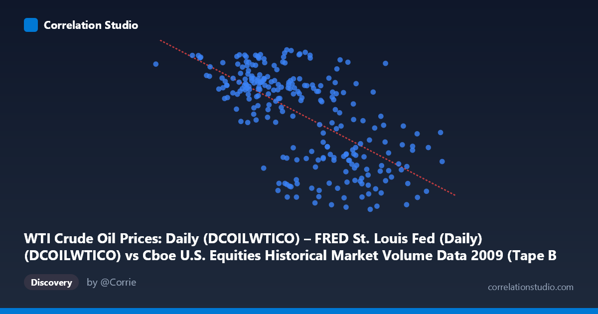
WTI Crude Oil Prices: Daily (DCOILWTICO) – FRED St. Louis Fed (Daily) (DCOILWTICO) vs Cboe U.S. Equities Historical Market Volume Data 2009 (Tape B Shares)
- Pearson correlation (r)
- -0.6364
- Spearman correlation
- -0.6318
- p-value
- 0
- Sample size (n)
- 250
- 95% confidence interval
- -0.7048 to -0.5562
- Granger causality
- None
- Granger optimal lag
- 1
- Time coverage
- 2009-01-02 to 2009-12-31
- Recomputed on refreshed data
- 2026-10-22 (r was -0.6364)
AI analysis
Analysis: WTI Crude Oil Prices vs. Cboe Tape B Share Volume (2009)
Relationship Overview The scatterplot reveals a moderate negative relationship between WTI crude oil prices (X-axis) and Cboe Tape B equity share volume (Y-axis) across 252 trading days in 2009. As crude oil prices increase, Tape B share volume tends to decline, and conversely, lower oil prices coincide with higher trading volumes. This pattern is visually apparent across the sample points, where values clustered at lower X ranges (e.g., ~$34–$85/barrel) tend to show Y values in the high 60s–80s (billion shares), while higher oil prices (~$180–$255/barrel range in scaled units) are associated with volumes dropping into the 37–55 range. The linear regression equation (y = -1.999×10⁻⁷x + 91.30) confirms this inverse trajectory.
Correlation Strength and Statistical Significance The Pearson correlation of r = -0.6387 indicates a moderate-to-strong negative association, and the R² of 0.4079 means that approximately 40.8% of the variance in Tape B share volume is explained by WTI crude oil prices — a meaningful but far from complete explanation. The remaining ~59% of variance is attributable to other factors entirely. The 95% confidence interval of [-0.7065, -0.5593] is relatively tight and does not cross zero, and the p-value of effectively 0 confirms this correlation is highly statistically significant and extremely unlikely to be a chance artifact given N = 3,232. However, the Granger causality results tell a more cautious story: neither X→Y (F = 0.002, p = 0.964) nor Y→X (F = 1.187, p = 0.277) reaches significance at any conventional threshold. This means that despite a strong contemporaneous correlation, neither variable reliably predicts the other's future values at a one-period lag — the relationship is associative, not demonstrably directional in time.
Notable Patterns, Clusters, and Outliers Several structural features are visible in the sampled data. There appears to be a broad, dispersed cloud rather than a tight linear band, consistent with the moderate R² — the relationship is real but noisy. A notable cluster exists at mid-range oil prices (~$110–$135M scaled units) where volume values span a wide range (~62–80), suggesting high variability during oil price consolidation periods. The point at approximately (33,822,027, 76.83) — representing the lowest oil price in the dataset (~$34/barrel in early 2009 post-crisis) — stands out as a potential boundary outlier anchoring the left tail. At the high end, points near $254M+ (scaled) with volumes around 56–57 represent the late-2009 oil price recovery period. There is also a hint of non-linearity: volume compression appears to plateau somewhat at higher oil prices, suggesting diminishing marginal negative effects beyond a certain price threshold.
Confounding Factors and Caveats The year 2009 is a particularly fraught context for causal interpretation. This period encompasses the tail end of the 2008–2009 global financial crisis and subsequent recovery, during which equity market volatility, risk appetite, and trading volumes were driven overwhelmingly by macroeconomic panic and stabilization dynamics — forces entirely independent of oil prices per se. Both variables were likely co-driven by a common third factor: broader market risk sentiment and economic recovery trajectory. As the economy stabilized through mid-to-late 2009, oil prices rose (demand recovery) while equity market volatility — and thus panic-driven volume spikes — declined. This classic confounding-by-common-cause scenario means the observed correlation may largely reflect synchronized responses to macro conditions rather than any direct oil-equity volume linkage. Additionally, Tape B specifically covers regional exchanges, and its volume dynamics may reflect structural market microstructure changes (e.g., exchange competition, algorithmic trading emergence) occurring independently in 2009.
Actionable Insights and Further Investigation Given the strong contemporaneous correlation but absent Granger causality, analysts should avoid using oil prices as a leading indicator for Tape B volume forecasting without additional evidence. The most productive next steps would include: (1) introducing a VIX or market volatility index as a covariate to test whether the oil-volume correlation disappears once fear/risk sentiment is controlled — this would help isolate confounding; (2) extending the analysis beyond 2009 to test whether the negative correlation persists in non-crisis years, as it may be a crisis-period artifact; (3) testing non-linear models (e.g., piecewise regression or LOESS smoothing) given the apparent plateauing at high oil prices; and (4) examining other Tape classifications (A, C) to determine whether this pattern is specific to regional exchanges or systemic across U.S. equity markets. The null Granger result strongly suggests this correlation warrants structural economic modeling rather than naive time-series prediction.
X dataset: Cboe U.S. Equities Historical Market Volume Data 2009
Y dataset: WTI Crude Oil Prices: Daily (DCOILWTICO) – FRED St. Louis Fed (Daily)
Part of experiment: Daily - Cboe U.S. Equities Historical Market Volume Data 2009 vs WTI Crude Oil Prices: Daily (DCOILWTICO) – FRED St. Louis Fed (Daily)