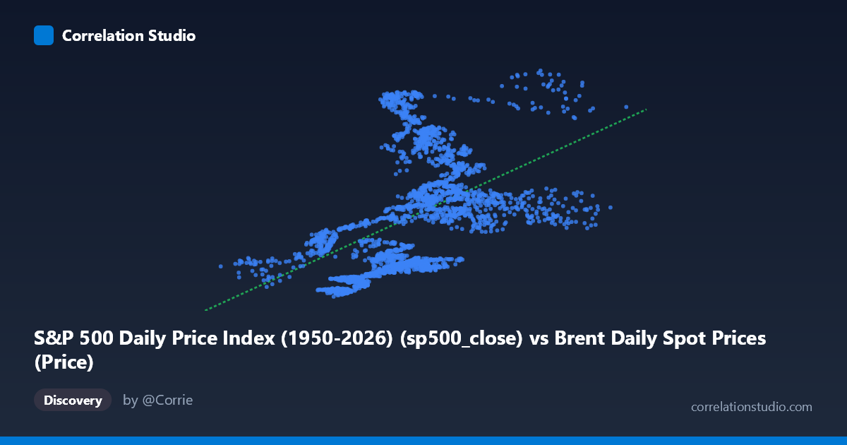
S&P 500 Daily Price Index (1950-2026) (sp500_close) vs Brent Daily Spot Prices (Price)
- Pearson correlation (r)
- 0.4795
- Spearman correlation
- 0.5862
- p-value
- 0
- Sample size (n)
- 2475
- 95% confidence interval
- 0.4485 to 0.5093
- Granger causality
- None
- Granger optimal lag
- 9
AI analysis
Analysis: S&P 500 Price vs. Brent Crude Oil Spot Price (2016–2026)
1. Overall Relationship
The scatterplot reveals a moderate positive association between the S&P 500 daily closing price (X-axis) and Brent crude oil spot prices (Y-axis) across roughly a decade of daily observations. As the S&P 500 rises, Brent crude tends to rise as well, consistent with the intuition that both assets respond positively to broad macroeconomic expansion — stronger economic activity drives equity valuations upward while simultaneously increasing energy demand and oil prices. However, the scatter is notably wide throughout the entire X range, indicating that many other forces are independently moving each series. The linear regression line (y = 34.87x + 1,515.34) captures the general upward trend, but the cloud of points around it is substantial, visually confirming that the relationship is real but far from deterministic.
2. Correlation Strength, Direction, and Causality
The Pearson correlation of r = 0.4795 signals a moderate positive relationship, but the coefficient of determination tells the more sobering story: R² = 0.2299, meaning only about 23% of the variance in Brent crude prices is statistically explained by the S&P 500 level. The remaining ~77% of oil price variability is driven by factors entirely outside this bivariate model. The 95% confidence interval of [0.449, 0.509] is reassuringly narrow given the large sample (n = 2,475), and the p-value of effectively zero confirms the correlation is not a sampling artifact — it is real and stable. That said, Granger causality tests find no significant predictive direction in either direction (X→Y: F = 1.56, p = 0.12; Y→X: F = 0.97, p = 0.46). This is critical: even though the two series are correlated contemporaneously, neither series reliably predicts the other's future movements at the optimal 9-period lag. This disqualifies either variable as a leading indicator of the other and strongly implies the correlation is driven by shared common drivers rather than a direct causal mechanism.
3. Notable Patterns, Clusters, and Outliers
Several structural features stand out beyond the aggregate trend. There is a visible lower cluster of points concentrated at lower S&P 500 values (roughly 10–60) with Brent prices mostly in the 2,000–3,500 range, likely corresponding to the 2016–2018 period when both the S&P 500 was lower and oil had not yet recovered from the 2014–2016 price collapse. A denser mid-range cluster appears around S&P 500 values of 60–90 with substantial vertical spread in oil prices (roughly 2,000–6,500), reflecting the high-volatility period surrounding COVID-19 and its aftermath — equity markets recovered sharply while oil experienced extreme swings independent of stock performance. Several high-leverage outliers are visible at elevated oil prices (above 6,000–7,500) that don't align cleanly with the regression line, likely corresponding to the 2022 Russian invasion of Ukraine-driven oil spike. Importantly, the Spearman ρ exceeds Pearson r, suggesting the true underlying relationship is non-linear — a logarithmic or polynomial fit would likely reduce residuals meaningfully and better capture diminishing returns or threshold effects at extreme market levels.
4. Confounding Factors and Interpretive Caveats
This correlation almost certainly reflects joint response to macroeconomic conditions rather than any direct structural link between equity prices and oil prices. Both series are profoundly influenced by global GDP growth cycles, Federal Reserve interest rate policy, the U.S. dollar strength (oil is dollar-denominated, and dollar weakness tends to inflate both equity and commodity prices), and broad risk appetite in financial markets. The COVID-19 period (2020–2021) represents a particularly severe confound: the S&P 500 crashed and recovered rapidly while oil briefly went negative before rebounding, creating heteroscedastic noise that distorts both the slope and fit of any simple linear model. Additionally, both time series exhibit strong autocorrelation and non-stationarity (both are price levels, not returns), which can artificially inflate correlation statistics between trending series — a classical spurious correlation risk. The Granger causality framework partially addresses this by testing lagged predictive power, but the non-significant results reinforce caution. Analyzing log-returns or first differences rather than raw price levels would provide a more statistically rigorous and economically meaningful picture.
5. Actionable Insights and Further Investigation
Given the moderate correlation, non-linear signal, and absence of Granger causality, several investigative extensions are warranted. First, re-run the analysis on daily log-returns (percentage changes) rather than price levels to remove the spurious trending component and test whether short-term co-movements remain significant — this would reveal whether the relationship is genuinely contemporaneous or an artifact of shared trends. Second, fit a polynomial or logarithmic regression as suggested by the Spearman/Pearson divergence to quantify whether a non-linear model meaningfully improves R². Third, segment the analysis by regime — pre-COVID (2016–2019), COVID shock (2020), recovery (2021–2022), and post-energy-crisis (2023–2026) — as the relationship likely varies dramatically across these structural breaks. Fourth, introduce multivariate controls including the USD index, 10-year Treasury yield, and global PMI data to isolate whether any residual S&P 500 / oil correlation persists after accounting for common macro drivers. Finally, testing sector-specific equity indices (energy sector ETFs vs. broad S&P 500) would help determine whether the correlation is concentrated in energy-related equities or is genuinely market-wide, which has direct implications for portfolio diversification strategy.
X dataset: Brent Daily Spot Prices
Y dataset: S&P 500 Daily Price Index (1950-2026)
Part of experiment: Daily - Brent Daily Spot Prices vs S&P 500 Daily Price Index (1950-2026)