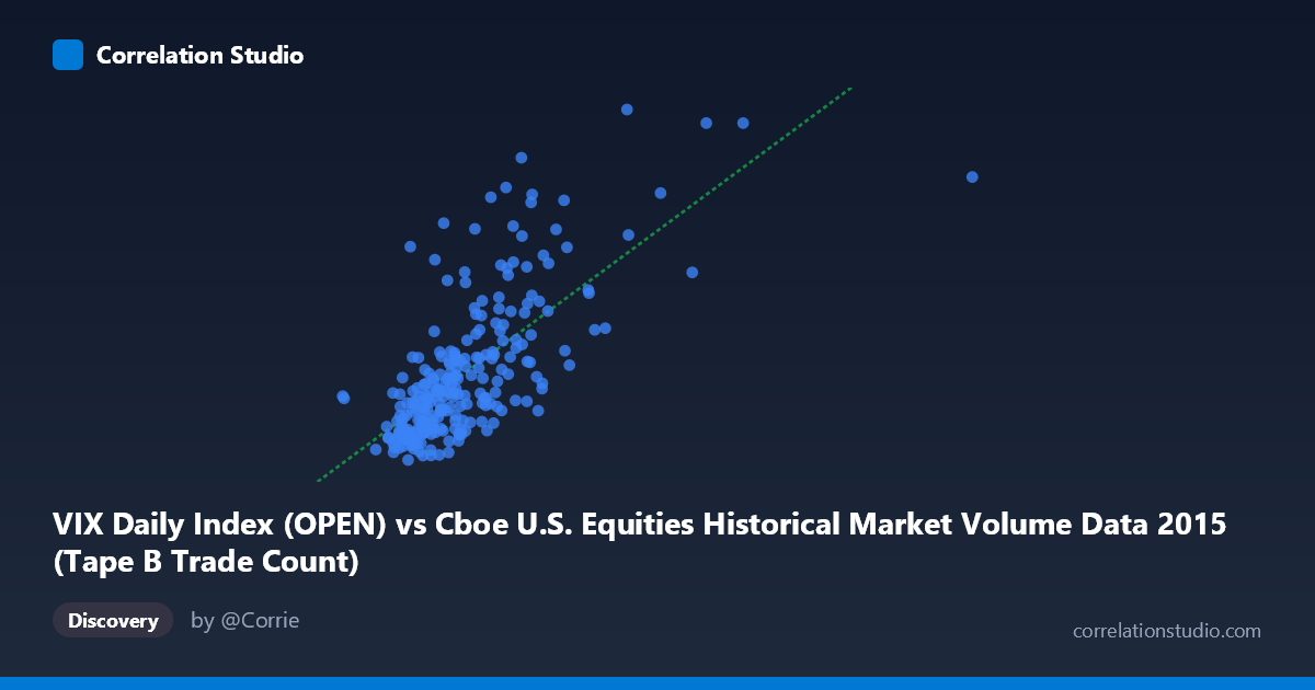
VIX Daily Index (OPEN) vs Cboe U.S. Equities Historical Market Volume Data 2015 (Tape B Trade Count)
- Pearson correlation (r)
- 0.7063
- Spearman correlation
- 0.7029
- p-value
- 0
- Sample size (n)
- 252
- 95% confidence interval
- 0.6384 to 0.7632
- Granger causality
- None
- Granger optimal lag
- 1
AI analysis
Analysis: VIX Daily Index (Open) vs. Tape B Trade Count
Relationship Overview
The scatterplot reveals a moderately strong positive relationship between the Cboe VIX Daily Index opening values and Tape B trade counts across U.S. equities exchanges in 2015. As VIX open levels rise — indicating greater expected market volatility — Tape B trade counts tend to increase correspondingly. This is intuitively consistent with market microstructure theory: elevated volatility environments typically drive higher trading activity as market participants rebalance portfolios, execute hedges, and respond to price uncertainty. The linear regression equation (y = 3.02×10⁻⁵x + 7.66) confirms a positive slope, though the relatively modest coefficient suggests the relationship, while real, is not dramatically steep across the observed range.
Correlation Strength and Statistical Significance
The Pearson correlation of r = 0.7063 indicates a moderately strong positive association, but the r² of 0.4988 is the more sobering statistic — only approximately 49.9% of variance in Tape B trade counts is explained by VIX open levels. This means roughly half the variation in trading activity remains attributable to other forces entirely. The 95% confidence interval of [0.6384, 0.7632] is reassuringly tight given the sample size of n = 252 drawn from a population of N = 3,302, and the p-value of effectively zero confirms the correlation is not a chance artifact. However, the Granger causality results are notably absent of significance in either direction — X→Y yields F = 0.014 (p = 0.906) and Y→X yields F = 0.448 (p = 0.504). This is a critical caveat: despite the strong contemporaneous correlation, neither variable meaningfully predicts the future values of the other at a one-period lag, meaning the relationship is associative rather than temporally directional.
Notable Patterns and Outliers
Several features stand out in the sample data. The bulk of observations cluster in the lower-left region, with VIX opens concentrated between roughly 130,000–400,000 and trade counts between 12–20, suggesting a relatively stable baseline trading regime for most of 2015. However, a meaningful number of high-leverage points exist in the upper-right quadrant — notably observations around (640,679; 31.13) and (621,009; 22.55) — which likely correspond to specific volatility episodes such as the August 2015 market selloff. The point (1,014,195; ~high Y) implied by the X-range maximum would be a significant outlier worth examining individually. There is also visible heteroscedasticity: variance in Y appears to fan outward as X increases, suggesting the linear model may underfit the high-volatility regime.
Confounding Factors and Caveats
Several confounds complicate causal interpretation. First, both variables are likely driven by common underlying market events — macro announcements, geopolitical shocks, or Federal Reserve communications — making shared causation from a third factor the most plausible explanation for their co-movement. Second, Tape B specifically covers NYSE American and regional exchange trades, which may respond differently to volatility than broader market measures. Third, the daily aggregation smooths intraday dynamics where the VIX-volume relationship is arguably strongest. The lack of Granger causality further underscores that the correlation is likely contemporaneous and event-driven rather than a predictive lead-lag structure, limiting its utility for forecasting applications.
Actionable Insights and Further Investigation
Practitioners should avoid using VIX opens as a standalone predictor of next-day Tape B volume given the failed Granger test. Instead, this relationship is better leveraged for same-day risk and capacity planning — elevated VIX opens could serve as a real-time signal to anticipate higher trade processing loads. Further investigation should include: (1) segmenting the data by volatility regime (e.g., VIX < 15 vs. 20) to test whether the relationship strengthens nonlinearly during stress periods; (2) adding additional explanatory variables such as S&P 500 returns, macro event dummies, or Tape A/C volumes to improve the r² beyond 50%; and (3) applying a rolling-window correlation analysis to assess whether the VIX–volume relationship was stable across 2015 or concentrated around specific episodes like the August correction.
X dataset: Cboe U.S. Equities Historical Market Volume Data 2015
Y dataset: VIX Daily Index
Part of experiment: Daily - Cboe U.S. Equities Historical Market Volume Data 2015 vs VIX Daily Index