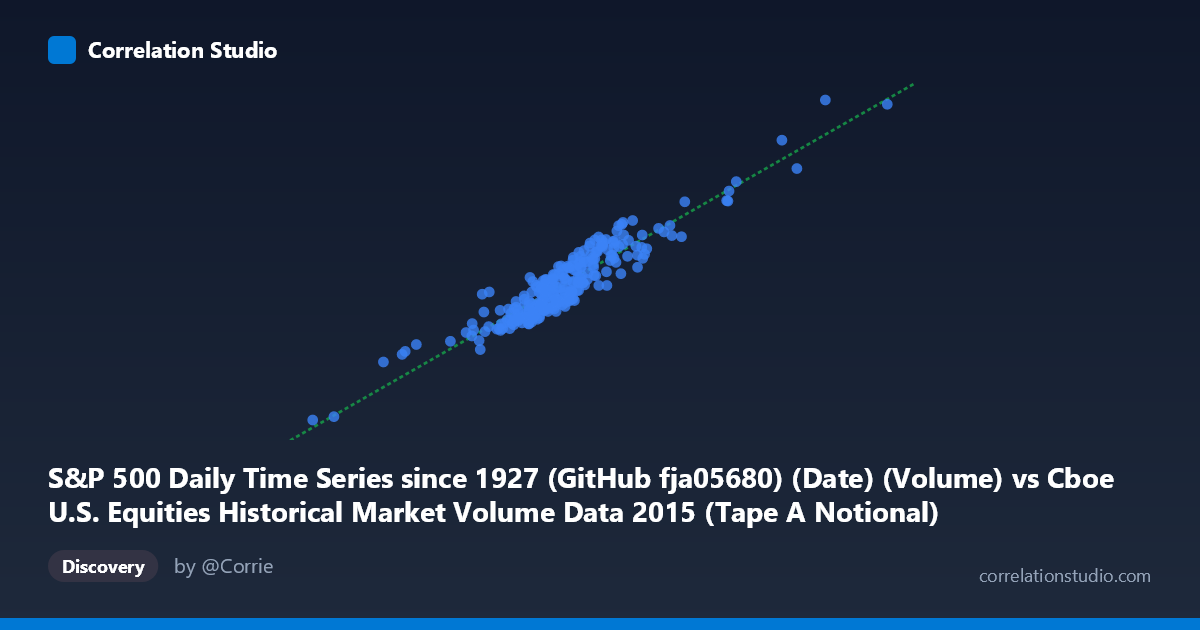
S&P 500 Daily Time Series since 1927 (GitHub fja05680) (Date) (Volume) vs Cboe U.S. Equities Historical Market Volume Data 2015 (Tape A Notional)
- Pearson correlation (r)
- 0.9366
- Spearman correlation
- 0.9095
- p-value
- 0
- Sample size (n)
- 252
- 95% confidence interval
- 0.9194 to 0.9502
- Granger causality
- None
- Granger optimal lag
- 10
AI analysis
Scatterplot Analysis: S&P 500 Trading Volume vs. Tape A Notional Value (2015)
Relationship Overview The scatterplot reveals a strong positive linear relationship between S&P 500 daily trading volume and Cboe Tape A notional value across 252 trading days in 2015. As daily share volume increases, the total notional dollar value of Tape A transactions rises commensurately, which is economically intuitive — more shares traded at prevailing market prices naturally generates higher notional turnover. The linear regression equation (y = 0.352x + 1.304×10⁸) suggests that for every additional share in volume, notional value increases by roughly $0.35, with a baseline intercept reflecting fixed structural activity in the market. The relationship appears reasonably tight across the central mass of observations, though with meaningful dispersion at higher volume levels.
Correlation Strength and Statistical Significance The Pearson correlation of r = 0.937 is exceptionally strong, and the coefficient of determination r² = 0.877 indicates that approximately 87.7% of the variance in Tape A notional value is explained by trading volume — a remarkably high figure for financial market data. The 95% confidence interval of [0.919, 0.950] is narrow and lies entirely in the high-positive range, confirming this is not a sampling artifact. The p-value of effectively zero, drawn from a paired sample of n = 252 against a population of N = 3,302, provides overwhelming statistical confidence that the correlation is real. However, the Granger causality results complicate the narrative significantly: neither direction (X→Y nor Y→X) reaches statistical significance at the optimal lag of 10 periods (F = 0.562, p = 0.844 and F = 0.631, p = 0.787, respectively). This means that while volume and notional value are tightly correlated contemporaneously, neither variable meaningfully predicts the other in a temporal, lead-lag sense — they move together rather than one driving the other forward in time.
Notable Patterns, Clusters, and Outliers The bulk of observations cluster in a relatively compact ellipse centered around the dataset means (~10.0B volume, ~$3.66B notional), consistent with normal trading conditions for most of 2015. However, several notable outliers emerge in the upper-right region of the chart — points with volumes exceeding ~12–14.5 billion and notional values approaching $5.0–6.7 billion. These likely correspond to high-volatility episodes in 2015, most plausibly the late-August market selloff driven by China growth fears, when U.S. equity markets experienced their largest single-day declines in years and volume surged dramatically. At the lower-left extreme, a clear outlier sits near (3.29B, $1.41B), representing an unusually quiet trading session — possibly a holiday-adjacent or low-liquidity day. The scatter also shows slight heteroscedasticity: variance in notional value visibly fans outward at higher volume levels, suggesting the relationship becomes less predictable during stress episodes.
Confounding Factors and Interpretive Caveats Several important caveats limit straightforward causal interpretation. First, the axes appear swapped in dataset labeling — the X-axis is labeled as a date column from the S&P 500 dataset being used as volume, and the Y-axis references Tape A notional from the Cboe dataset, suggesting possible metadata misalignment that warrants verification. Second, notional value is mechanically related to volume through price (Notional ≈ Volume × Price), meaning this correlation is partly tautological — a rising price environment alone inflates notional value even at constant volume. Since 2015 saw meaningful intra-year price swings in the S&P 500 (roughly −12% peak-to-trough), price level acts as a significant confounder. Third, Tape A covers only NYSE-listed securities, so the relationship captures a subset of total market activity; structural shifts in exchange market share during 2015 could distort the relationship. Finally, the lack of Granger causality despite high contemporaneous correlation strongly implies a common driver (e.g., market volatility, macro news events) is simultaneously influencing both series.
Actionable Insights and Further Investigation Practitioners should not use volume to forecast next-day notional value (or vice versa) given the failed Granger tests — the predictive value is contemporaneous only, limiting tactical utility. To deepen understanding, analysis should: (1) partial out price-level effects by examining volume vs. notional value normalized by the daily S&P 500 closing price, which would test whether the relationship holds beyond arithmetic identity; (2) segment the data by volatility regime (e.g., VIX above/below 20) to determine whether the correlation structure differs during stress periods, particularly given the visible upper-tail outliers; (3) extend the time series beyond 2015 to test whether this correlation is stable across different market cycles (2020 COVID volatility, 2022 rate-shock environment); and (4) investigate whether intraday volume distribution or specific Tape A participant types (market makers vs. institutional) drive the outlier sessions differently from normal days.
X dataset: Cboe U.S. Equities Historical Market Volume Data 2015
Y dataset: S&P 500 Daily Time Series since 1927 (GitHub fja05680) (Date)
Part of experiment: Daily - Cboe U.S. Equities Historical Market Volume Data 2015 vs S&P 500 Daily Time Series since 1927 (GitHub fja05680) (Date)