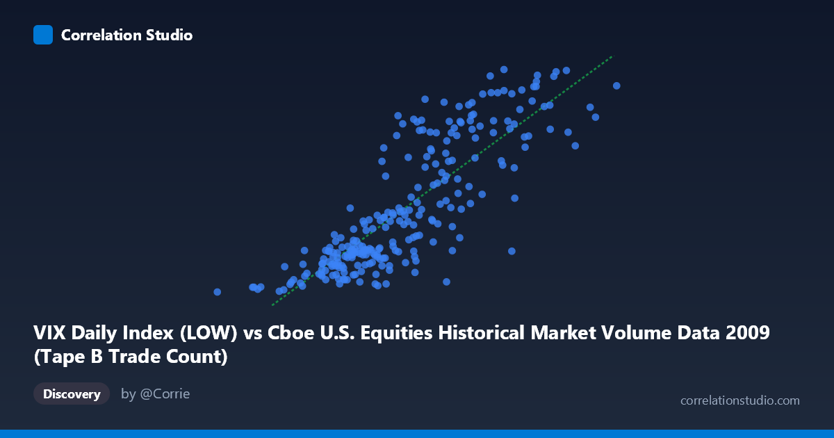
VIX Daily Index (LOW) vs Cboe U.S. Equities Historical Market Volume Data 2009 (Tape B Trade Count)
- Pearson correlation (r)
- 0.8343
- Spearman correlation
- 0.8418
- p-value
- 0
- Sample size (n)
- 252
- 95% confidence interval
- 0.7924 to 0.8683
- Granger causality
- None
- Granger optimal lag
- 1
AI analysis
Scatterplot Analysis: VIX Daily Index (LOW) vs. Tape B Trade Count (2009)
Relationship Overview The scatterplot reveals a moderately strong positive relationship between the VIX Daily Index Low values and the Cboe U.S. Equities Tape B Trade Count across 2009. As the VIX low increases — indicating higher baseline volatility — trade counts on Tape B rise correspondingly. This is conceptually intuitive: elevated volatility environments tend to drive greater trading activity as market participants react to uncertainty, hedge positions, and rebalance portfolios. The linear regression equation (y = 5.76×10⁻⁵x + 7.34) confirms this positive slope, and the visual distribution of points broadly follows this upward trajectory.
Correlation Strength and Statistical Interpretation The correlation coefficient of r = 0.8343 indicates a strong positive association, and the R² of 0.696 means that approximately 69.6% of the variance in Tape B trade counts is explained by the VIX low level — a substantial explanatory share for financial market data. The 95% confidence interval of [0.79, 0.87] is relatively tight, reflecting the reasonably large paired sample of n = 252, and the p-value of essentially zero confirms the relationship is highly unlikely to be a statistical artifact. However, the Granger causality results tell a more cautious story: neither direction (X→Y: F = 0.009, p = 0.92; Y→X: F = 0.036, p = 0.85) reaches significance at lag-1, meaning that despite the strong contemporaneous correlation, neither variable reliably predicts the other's next-period movement. This is a critical distinction — the variables move together, but one does not temporally lead the other in a predictive sense.
Patterns, Clusters, and Outliers The scatterplot exhibits a discernible clustering pattern rather than a uniform distribution. A dense cluster of points occupies the lower-left region (VIX low ~80,000–400,000; trade counts ~19–26), corresponding likely to the more stable mid-year months of 2009 as markets recovered from the financial crisis lows. A second, more dispersed cluster appears in the upper-right (VIX low ~500,000–770,000; trade counts ~40–49), reflecting the high-volatility, high-volume period likely concentrated in early 2009. Several points near the extremes — particularly the observations around (766,764, 47.08) and (629,100, 47.65) — appear as potential high-leverage points that could disproportionately influence the regression fit. The bimodal distribution of data also hints at possible non-linearity or regime-switching behavior rather than a clean linear relationship across the full range.
Confounding Factors and Caveats Several important caveats limit causal interpretation here. First, 2009 is an unusual year — it spans the tail of the global financial crisis and a sharp market recovery, meaning both VIX and trading volumes were driven by the same underlying macro shock (the crisis itself), making them spuriously correlated via a common cause. Second, Tape B specifically covers NYSE American and regional exchange stocks, so trade count dynamics may reflect structural factors (e.g., exchange routing changes, algorithmic activity) independent of volatility. Third, the axes appear swapped relative to the source dataset descriptions — the VIX variable appears on the X-axis despite originating from the market volume dataset, and Tape B counts on the Y-axis from the VIX dataset, suggesting a data labeling irregularity that warrants verification before drawing firm conclusions. Finally, the absence of Granger causality undermines any narrative about one variable driving the other.
Actionable Insights and Further Investigation Given the strong contemporaneous correlation but absent temporal predictability, the most productive next steps would be: (1) extending the analysis beyond 2009 to test whether the relationship holds across different volatility regimes, or whether it is a crisis-period artifact; (2) introducing macro controls such as S&P 500 returns or credit spreads to partial out the common crisis driver; (3) testing non-linear models (e.g., piecewise regression or quantile regression) given the apparent bimodal clustering; and (4) examining intraday data to assess whether very short-lag Granger effects exist that daily data obscures. Practitioners should treat this correlation as a useful descriptive co-movement signal rather than a predictive trading rule, given the Granger causality null result.
X dataset: Cboe U.S. Equities Historical Market Volume Data 2009
Y dataset: VIX Daily Index
Part of experiment: Daily - Cboe U.S. Equities Historical Market Volume Data 2009 vs VIX Daily Index