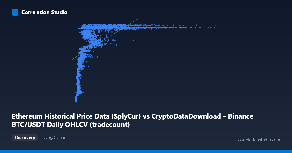
Ethereum Historical Price Data (SplyCur) vs CryptoDataDownload – Binance BTC/USDT Daily OHLCV (tradecount)
- Pearson correlation (r)
- 0.5542
- Spearman correlation
- 0.8316
- p-value
- 0
- Sample size (n)
- 3191
- 95% confidence interval
- 0.5296 to 0.5777
- Granger causality
- X → Y
- Granger optimal lag
- 10
AI analysis
Analysis: Relationship Between Ethereum Supply Metric and BTC/USDT Trade Count
1. Overview of the Relationship
The scatterplot depicts a positive but non-linear association between the X variable (labeled as Ethereum's circulating supply, though the values and range suggest this may actually be a mislabeled price/volume-type metric) and the Y variable (tradecount). The data shows a distinctive curved pattern: Y values rise steeply from ~94M to ~120M as X increases from near-zero to roughly 1-2 million, then plateau — with most of the mass sitting in a saturated band near 120-121M once X exceeds ~2 million. This shape strongly resembles a logarithmic or saturating growth curve rather than a straight line.
2. Correlation Strength, Uncertainty, and Causality
The Pearson correlation (r = 0.554) indicates a moderate positive relationship, with r² = 0.307 meaning the linear model explains only about 31% of the variance in Y — leaving nearly 70% unexplained by a straight-line fit. The 95% CI [0.530, 0.578] is tight given the large sample (n = 3,191), and the p-value of ~0 confirms the correlation is highly statistically significant — but statistical significance here reflects sample size more than practical linear strength. Critically, the note that Spearman's ρ exceeds Pearson's r confirms the visual impression: a monotonic but curved (likely logarithmic) relationship fits better than the linear model, meaning the true explanatory power is understated by r². On causality, Granger tests show X→Y is significant (F=2.18, p=0.016) at a 10-period lag, while Y→X is not (p=0.765), suggesting X's past values have modest predictive value for future Y, but not vice versa — though with F≈2.18, this is a weak-to-moderate effect, not a dominant driver.
3. Notable Patterns and Outliers
The chart's most salient feature is the "hockey-stick" or logistic-like curve: a steep rise for small X (under ~1M) transitioning into a flat ceiling near Y≈120-121M for larger X. This creates two visual clusters — a scattered "ramp" of points with lower Y (94M-118M) at low X, and a dense horizontal band at high Y for X 2M. A few low-X, low-Y points (e.g., X≈2,000-10,000, Y≈94M) stand out as an initial "floor," likely representing early time periods (2017-2018) before tradecount scaled up. The extreme X outliers (up to 15.3M, far beyond the mean of ~2M plus ~6.5 stdev) pull heavily on any linear fit despite contributing little additional Y variance, which also helps explain the modest r².
4. Confounding Factors and Caveats
Since this spans 2017-2026, both series are likely non-stationary time series with trends driven by overall crypto market maturation (exchange volume growth, adoption, bull/bear cycles) rather than a direct causal mechanism between the two specific metrics. This raises strong concern for spurious correlation via a shared time trend — both variables may simply be trending upward with market growth independently. The mismatched/ambiguous variable labeling (Ethereum "SplyCur" vs. BTC/USDT tradecount from a different dataset) also warrants a data-provenance check, as pairing unrelated exchange/dataset metrics can produce misleading correlations. Additionally, the saturation plateau suggests Y has a practical ceiling (possibly a data cap or reporting limit) that mechanically weakens correlation for large X.
5. Recommendations
1. Refit with a log or logistic model: Given Spearman Pearson and the visible curve, try y = a·ln(x) + b or a saturating/logistic function — this should substantially raise explained variance beyond 30.7%. 2. Detrend or difference the series before correlation/Granger analysis to rule out shared-trend spuriousness — test correlation on returns/changes rather than levels. 3. Verify variable/dataset alignment — confirm that X (Ethereum SplyCur) and Y (BTC/USDT tradecount) are correctly paired by timestamp and that labels/units are accurate. 4. Investigate the low-X cluster separately (likely early 2017-2018 data) as a distinct regime, since pooling it with later high-X data may distort both the linear fit and causality tests. 5. Extend Granger analysis with control variables (e.g., overall market volume or BTC price) to check if the X→Y predictive signal survives after controlling for common market-wide drivers.
X dataset: CryptoDataDownload – Binance BTC/USDT Daily OHLCV
Y dataset: Ethereum Historical Price Data
Part of experiment: Bitcoin - CryptoDataDownload – Binance BTC/USDT Daily OHLCV vs Ethereum Historical Price Data