S&P 500 Daily Time Series since 1927 (GitHub fja05680) (Date) (Volume) vs Cboe U.S. Equities Historical Market Volume Data 2013 (Tape A Notional)
- Pearson correlation (r)
- 0.9399
- Spearman correlation
- 0.8898
- p-value
- 0
- Sample size (n)
- 252
- 95% confidence interval
- 0.9236 to 0.9528
- Granger causality
- None
- Granger optimal lag
- 10
AI analysis
Analysis: S&P 500 Trading Volume vs. Tape A Notional Value (2013)
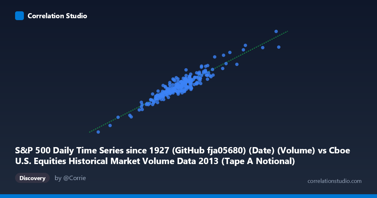
Relationship Overview The scatterplot reveals a strong, positive linear relationship between total U.S. equities market volume (X-axis, measured in shares traded) and Tape A notional value (Y-axis, measured in dollars). As daily trading volume increases, the dollar value of Tape A transactions rises correspondingly. The linear regression equation y = 0.4374x + 2.084×10⁸ describes this relationship well, with the slope indicating that each additional share of volume is associated with roughly $0.44 in Tape A notional value — reflecting the average price weighting of NYSE-listed securities in the broader market mix. The data spans the full 2013 trading calendar (252 business days), providing a complete annual picture with no obvious seasonal gaps.
Correlation Strength and Statistical Significance The correlation is exceptionally strong (r = 0.9399), and the R² of 0.8834 means that 88.3% of the day-to-day variance in Tape A notional value is explained by total market volume alone — a remarkably high figure for financial market data. The 95% confidence interval [0.9236, 0.9528] is narrow, indicating high precision in this estimate, and the p-value of effectively zero confirms this is not a chance association across the n=252 paired observations. However, Granger causality tests reveal no significant predictive directionality in either direction (X→Y: F=1.013, p=0.433; Y→X: F=0.925, p=0.511) at the optimal 10-period lag. This is a critical nuance: while the two variables move together strongly in contemporaneous terms, neither one meaningfully predicts the other across subsequent trading days, suggesting they are co-driven by the same underlying market forces rather than one leading the other.
Notable Patterns, Clusters, and Outliers The sample points reveal a moderately tight central cluster concentrated roughly around X ≈ 6.5–8.5 billion shares and Y ≈ 3.0–3.9 billion dollars in notional value, consistent with the mean values (X̄ ≈ 7.20B, Ȳ ≈ 3.36B). A few notable outliers are visible at the extremes: the point near (3.99B, 1.97B) and another near (4.60B, 2.05B) represent unusually low-volume days far from the main cluster — likely holiday-adjacent sessions or summer doldrums. At the upper end, points such as (9.01B, 4.66B) and (8.43B, 3.95B) represent high-conviction market days, possibly coinciding with macro events like FOMC announcements or index rebalancing. One potentially anomalous point, (7.52B, 4.08B), sits notably above the regression line, suggesting an elevated notional value relative to volume — perhaps a day dominated by high-priced large-cap NYSE trading.
Confounding Factors and Interpretive Caveats Several confounds warrant caution. Tape A notional value is not independent of price levels — it reflects both volume and prevailing stock prices, meaning that a rising market in 2013 (the S&P 500 gained ~30% that year) would mechanically inflate notional values even on days with flat volume. This price-level effect likely inflates the correlation and conflates two distinct phenomena: activity intensity and valuation drift. Additionally, Tape A covers only NYSE-listed securities, so the X-axis (total market volume including Tapes B and C) is a broader measure — the strong correlation may partly reflect a stable structural composition of the market rather than a behavioral relationship. The Granger causality null result also cautions against any trading strategy inference, as the variables cannot be used to forecast one another over subsequent sessions.
Actionable Insights and Further Investigation For market microstructure researchers, the strong contemporaneous correlation with no Granger causality suggests these metrics are best treated as coincident indicators of market activity rather than leading/lagging signals. A natural next step would be to decompose the residuals — the ~11.7% of unexplained variance — to identify whether outlier days cluster around specific event types (earnings seasons, Fed meetings, VIX spikes). It would also be valuable to partial out the S&P 500 price index level as a covariate to isolate pure volume effects from price-driven notional inflation. Extending the analysis across multiple years (the dataset dates to 1927) could test whether this structural relationship is stable across different volatility regimes or breaks down during crisis periods like 2008–2009. Finally, comparing Tape A with Tapes B and C separately could reveal whether the relationship holds uniformly or whether certain exchange segments drive the correlation disproportionately.
X dataset: Cboe U.S. Equities Historical Market Volume Data 2013
Y dataset: S&P 500 Daily Time Series since 1927 (GitHub fja05680) (Date)
Part of experiment: Daily - Cboe U.S. Equities Historical Market Volume Data 2013 vs S&P 500 Daily Time Series since 1927 (GitHub fja05680) (Date)